How exact input uncertainty becomes output uncertainty, why local and finite sensitivity differ, and why a good solver cannot cure an ill-conditioned problem.
Numerical conditioning
Numerical conditioning describes how sensitive the exact solution of a mathematical problem is to small changes in its input data. A problem is well-conditioned when the permitted small input changes produce small output changes on the chosen scale. It is ill-conditioned when some of those changes produce much larger output changes.
That distinction matters before a quant chooses a solver. Nearly redundant hedge instruments, closely related regression factors and weakly identified calibration parameters can turn modest data uncertainty into large movements in the answer. A more accurate calculation can expose that sensitivity; it cannot remove the uncertainty in the inputs.
A small change, computed exactly
Take the synthetic, dimensionless map
f(x)=1−x1,x=1.
At x=0.99, the exact output is 100. Increase the input by h=0.0001, giving x+h=0.9901. The new exact output is
f(0.9901)=9910000≈101.010101.
Measure both changes relative to their original values:
Quantity
Exact relative change
Percentage change
Input
0.0001/0.99=1/9900
Approximately 0.010101%
Output
(10000/99−100)/100=1/99
Approximately 1.010101%
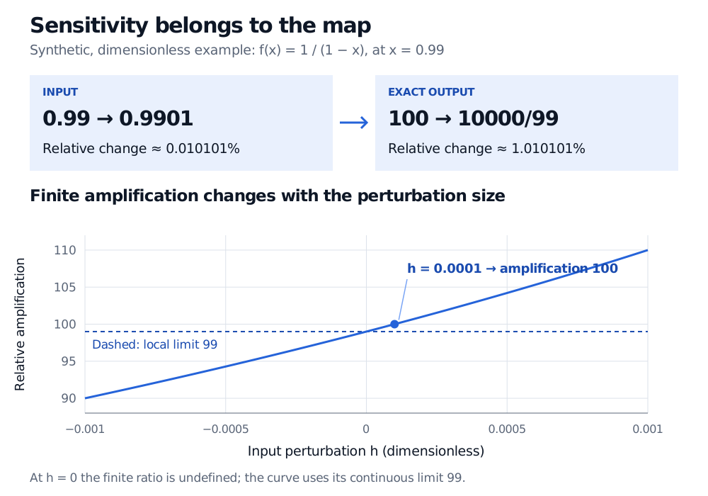
The ratio of the relative changes is 100. These are exact rational calculations, with rounding only in the displayed decimals. No floating-point failure is needed to explain the amplification: the mathematical map itself becomes sensitive as its denominator approaches zero.
For f(x)=1/(1-x) at x=0.99, an input increase of 0.0001 produces relative amplification 100. The finite amplification curve ranges from 90 to 110 for h from -0.001 to 0.001, while its local limit is 99.
Original synthetic example, evaluated in exact rational arithmetic. The solid curve shows relative amplification for finite perturbations; the dashed line shows its limit as the perturbation tends to zero.
Why the local condition number is 99
For a differentiable scalar map, the local absolute condition number is
κabs(x)=∣f′(x)∣.
It measures output change per unit of input change. When x=0 and f(x)=0, the corresponding local relative condition number is
κrel(x)=f(x)xf′(x).
For the example, f′(x)=1/(1−x)2, so at x=0.99 the absolute condition number is 10000 and the relative condition number is 99. A first-order approximation predicts an output increase of 10000h=1, or 1% of the original output. The exact finite increase is slightly larger.
There is no contradiction between local 99 and finite 100. For this map, direct subtraction gives, when h=0 and both outputs exist,
∣h∣/∣x∣∣f(x+h)−f(x)∣/∣f(x)∣=1−x−hx.
At x=0.99 and h=0.0001, that ratio is 100; as h→0, it tends to 99. The derivative describes infinitesimal changes, not a universal exact multiplier for every finite perturbation. A finite error bound needs control over the relevant neighbourhood.
A solver can converge while the answer remains uncertain
Numerical stability concerns the computational procedure. Conditioning concerns the exact input-to-answer map, with the inputs, permitted perturbations and error scale specified. A backward-stable method returns the exact answer to a nearby problem. If nearby problems have very different answers, a small backward error can coexist with a substantial forward error.
Consider implied volatility. Hold the other pricing inputs fixed and write an option price as C(σ). At an interior solution with nonzero vega, inverse differentiation gives
dCdσ=∂C/∂σ1,δσ≈∂C/∂σδC.
Here volatility is in annualised decimal units and vega is price change per unit of that volatility; a quote of vega per percentage point must be converted consistently. Small vega makes the inverse sensitive in absolute terms: a narrow price uncertainty can correspond to a wide volatility uncertainty. Tightening the root-finder's tolerance reduces its computational error but does not narrow the original quote uncertainty. The local formula also requires a sufficiently small perturbation; a price near a model boundary needs separate care.
The SelfMadeQuant lesson Numerical Conditioning and Stability develops the same distinction for linear hedge systems and covariance calculations. The full lesson requires membership; a public preview is available.
Choose the scale before judging the answer
Relative conditioning depends on dividing by the original output. Near zero, a large relative change may describe an economically small absolute change; at a zero output, the ordinary relative definition is undefined. A nearly delta-neutral portfolio, for example, needs a tolerance in meaningful exposure units rather than a percentage of zero.
Report the input uncertainty, the sensitivity of the requested output, and the numerical error separately. Use absolute error or an explicitly chosen reference scale when relative error loses its meaning. In vector problems, also state which inputs may move and how their sizes are measured: a condition number for perturbing quotes is not automatically a condition number for perturbing a covariance matrix or for normalised portfolio weights.
Sources
Lloyd N. Trefethen and David Bau III, Numerical Linear Algebra, SIAM, 1997, Lecture 12, “Conditioning and Condition Numbers,” and Lecture 14, “Stability.”
John C. Hull, Options, Futures, and Other Derivatives, ninth Global Edition, Pearson, 2018, Sections 15.11 (implied volatilities) and 19.8 (vega).