Find the input that makes a pricing residual zero, compare bisection with Newton, and distinguish a small price mismatch from a reliable yield-error bound.
Root-finding
Root-finding is the task of finding an input x∗ for which a function equals zero: f(x∗)=0. An equation such as “model price equals observed price” becomes a root problem by moving everything to one side. A numerical root-finder returns an approximation, together with evidence that it meets the requested accuracy.
This reverses a familiar financial calculation. Pricing starts with a yield and produces a bond price; root-finding starts with a price and recovers a yield to maturity. Recovering implied volatility from an option quote follows the same pattern, although its domain and derivative differ.
A yield hidden inside a price
Consider a hypothetical zero-coupon bond. It costs USD 80 today and pays USD 100 exactly two years later, with no interim payments. Use an annual effective yieldy, in decimal form. Assume full payment, ignore fees and taxes, and take two years as the specified year fraction; no calendar day-count conversion is needed. The price input is the total settlement amount for the claim, without an extra accrued-interest adjustment.
The domain requires a positive annual accumulation factor. The mathematical formula also has a negative-base solution outside this domain; it is inadmissible under the stated yield convention. A positive residual means the model price is too high; a negative residual means it is too low. Its units are USD per bond, while the unknown is an annual rate.
Here an analytic solution provides a useful benchmark:
y∗=80100−1=0.1180339887…≈11.803399%.
A numerical solver is unnecessary for this particular bond. The example lets us check the procedure before using it on a coupon schedule or valuation model that is harder to invert. Changing to continuous compounding would change both the price equation and the numerical yield quote.
A bracket proves something a guess cannot
At two candidate yields,
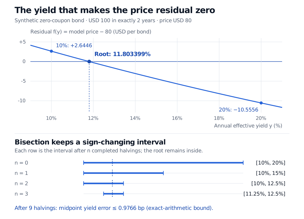
f(0.10)≈+2.6446,f(0.20)≈−10.5556.
Because f is continuous throughout 0.10,0.20], the [intermediate value theorem guarantees at least one root between the endpoints. This interval is a sign-changing bracket. Check endpoint values; a plausible-looking yield range is not automatically a bracket. An endpoint already satisfying f=0 can be returned directly.
Existence and uniqueness are separate questions. In this example,
f′(y)=−(1+y)3200<0(y>−1),
so the residual is strictly decreasing: there can be at most one admissible root. Together, the sign change and monotonicity establish exactly one. General root problems may have several roots, and one successful solve does not enumerate them.
The bisection method evaluates the midpoint and retains a half-interval whose endpoints still have opposite signs. For this decreasing residual:
Midpoint yield
Residual, USD per bond
Retained bracket
15%
−4.3856
[10%, 15%]
12.5%
−0.9877
[10%, 12.5%]
11.25%
+0.7979
[11.25%, 12.5%]
For a synthetic two-year bond paying USD 100 and costing USD 80, the residual falls from plus USD 2.6446 at 10% annual effective yield to minus USD 10.5556 at 20%, crossing zero at 11.803399%. Bisection retains brackets 10–20%, 10–15%, 10–12.5% and 11.25–12.5%. After nine halvings the midpoint error bound is 0.9766 basis points.
Original synthetic bond example. The upper panel shows the price mismatch; the lower panel shows intervals containing the yield. These measure different kinds of error.
Bisection does not require monotonicity to retain a root. Continuity and opposite endpoint signs suffice; monotonicity helps establish uniqueness. Conversely, opposite signs without continuity are insufficient: 1/x changes sign between −1 and 1 but has no root and is undefined at zero. Nor does every root change sign: (x−1)2 touches zero at 1. A scan for sign changes can miss such a repeated root.
How close is close enough?
Two tolerances answer different questions:
Residual tolerance: is ∣f(y^)∣ acceptably small in USD per bond?
Root tolerance: is ∣y^−y∗∣ acceptably small in decimal yield, perhaps expressed in basis points? One basis point is 0.0001 in decimal yield.
After n completed bisection halvings of an initial bracket [a0,b0], its current midpoint mn satisfies the exact-arithmetic bound
∣mn−y∗∣≤2n+1b0−a0.
Starting with width 0.10, nine halvings give a midpoint bound of 0.00009765625, or 0.9765625 basis points. This certificate depends on preserving a genuine bracket and reliably evaluating signs. Floating-point arithmetic can eventually prevent further subdivision.
A small residual alone gives no universal bound on root error. For example, g(x)=10−12(x−1) has residual 10−12 at x=2, yet the root error is 1. Multiplying an equation by a small constant changes its residual scale without moving its root.
A slope bound supplies the missing link. If y^ and y∗ lie in an interval where f is differentiable and ∣f′(y)∣≥m>0, the mean value theorem gives
∣y^−y∗∣≤m∣f(y^)∣.
For our bond on [0.10,0.20], the smallest slope magnitude is m=200/1.23=115.740740…USD per unit of decimal yield. Thus a residual no larger than USD 0.01 implies yield error no larger than 0.864 basis points, provided the candidate remains in this interval. Without a valid slope lower bound, dividing by one observed slope is only a local error estimate. Flat curves make inverse problems sensitive.
These are numerical guarantees for the specified equation. They do not remove price uncertainty, default risk or model error. With noisy simulation prices, unreliable residual signs can invalidate a bracket update; requesting precision below the valuation noise does not solve that problem.
Starting at 20% in the bond example produces decimal yields 0.1088, 0.1179199066 and 0.1180339713. The first step overshoots to the other side of the root; subsequent steps approach it rapidly. For a sufficiently smooth function near a simple root with nonzero derivative and a sufficiently close start, Newton has quadratic convergence: the error is approximately proportional to the previous error squared.
Method
Useful strength
Cost or limitation
Bisection
Derivative-free; shrinking bracket gives an error bound
Predictable but slower interval reduction; needs a continuous sign-changing bracket
Newton
Often very fast near a simple root
Needs a derivative and a suitable start; may leave the domain, cycle or fail
Safeguarded Newton
Uses a bracket while trying faster tangent steps
Must reject unsuitable steps and enforce enough bracket reduction
A practical safeguard keeps a valid bracket, rejects nonfinite, out-of-domain or unhelpful Newton candidates, and takes a bisection step when necessary. Merely accepting every candidate inside the bracket is not enough to ensure a useful rate of progress. Brent's method offers another bracketed approach using interpolation and bisection; it does not require a Newton derivative.
Choose tolerances in stated units. Combining an absolute rate tolerance with a relative one is useful across scales; near zero yield, an absolute tolerance is essential. Set an iteration limit and treat nonfinite evaluations or exhausted iterations as failures, rather than returning an unchecked rate.
For a broader treatment of finance roots alongside numerical integration, see Root-Finding and Numerical Integration. Its public page provides a preview; the full lesson requires membership.
Sources
James Stewart, Single Variable Calculus: Early Transcendentals, 6th edition, §4.8, “Newton's Method” — tangent iteration and failure from unsuitable starting points.
John C. Hull, Options, Futures, and Other Derivatives, 9th Global Edition, §§4.3–4.4 and the bond-yield Newton footnote — zero rates, price–yield inversion and compounding conventions. The worked bond here uses annual effective compounding.