Newton-Raphson finds a root by following tangent intercepts. Work through a bond yield, understand local quadratic convergence, and distinguish residual, step and yield-error tolerances.
Newton-Raphson method
The Newton–Raphson method, also called Newton's method, is an iterative root-finding algorithm: it approximates a solution of f(x)=0 by repeatedly replacing the curve with its tangent line and taking that line's zero as the next guess. It uses both the function value and its derivative:
xn+1=xn−f′(xn)f(xn).
The attraction in finance is inversion. A pricing formula takes a yield or volatility and returns a price; a desk often has the price and needs the parameter. Newton turns the price mismatch into a proposed parameter correction. That correction can be very effective near a well-behaved solution, but it does not guarantee a valid next guess or convergence.
Why the tangent gives this step
At the current guess xn, the tangent approximation is
f(x)≈f(xn)+f′(xn)(x−xn).
Set the right-hand side to zero and solve for x. The result is the Newton update above. The ratio f/f′ has the units of the unknown: if the residual is measured in dollars and the derivative in dollars per unit of decimal yield, the correction is a decimal yield, not a percentage-point number to insert unchanged into a percentage display.
A nonzero derivative is essential for the division. Even then, the tangent is only a local approximation. Its intercept is a candidate that must be evaluated in the original function on the next iteration.
Recovering a yield from a bond price
Consider a hypothetical zero-coupon bond costing USD 80 today and paying USD 100 exactly two years later, with no interim payments. Ignore default, taxes and fees. Let y be its annual effective yield to maturity, expressed as a decimal, with admissible domain y>−1. Define
f(y)=(1+y)2100−80,f′(y)=−(1+y)3200.
A positive residual means the model price exceeds the target price. Because the derivative is negative, the Newton correction then raises the yield and lowers the model price.
Start at y0=0.10. The first step is
y1=0.10−−150.262960180…2.644628099…=0.1176.
Iteration n
Yield yn, annual effective
Price residual f(yn), USD
0
10.0000000000%
2.644628099
1
11.7600000000%
0.062143595
2
11.8033736090%
0.000036158
3
11.8033988750%
1.226×10⁻¹¹
Numbers are rounded for display; the iterations use unrounded values. This bond also has an analytical solution,
y∗=80100−1=0.1180339887498948…,
which makes it possible to check the algorithm independently. A coupon bond usually requires a numerical solve because several discounted payments enter the price equation.
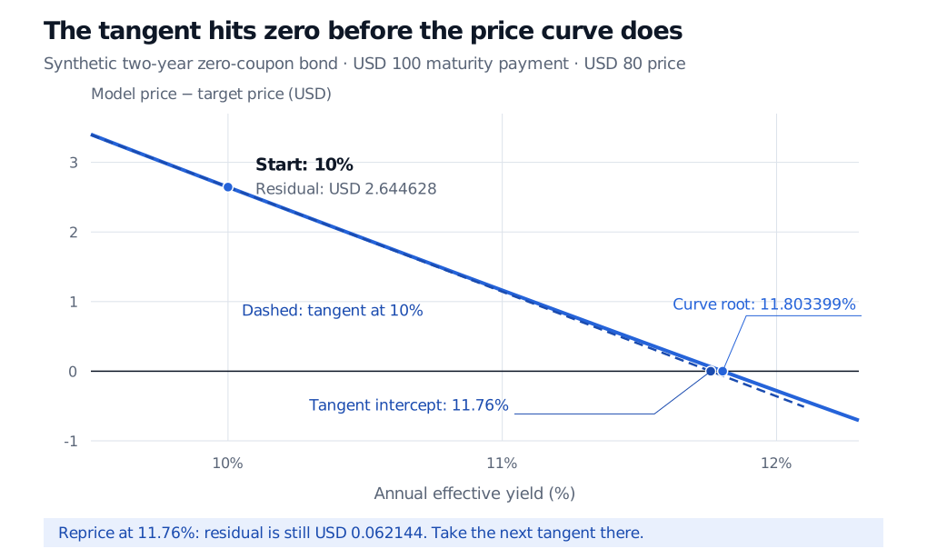
For a synthetic two-year zero-coupon bond paying USD 100 and priced at USD 80, the price residual at a 10% annual effective yield is USD 2.644628. Its tangent reaches zero at 11.76%, where the true residual is still USD 0.062144. The curve reaches zero at 11.803399%.
Original synthetic example. The dashed tangent proposes 11.76%; the blue curve must be evaluated again at that yield. Rates use annual effective compounding.
The root is unique here because f is continuous and strictly decreasing on y>−1, approaches positive infinity as y approaches −1 from above, and tends to −80 as y increases without bound. Uniqueness comes from the equation's structure; Newton itself does not establish it.
Fast convergence has local conditions
Suppose f is twice continuously differentiable near a root r, and f′(r)=0, so the root is simple. For a sufficiently close initial guess, Newton converges locally with an error bound of the form
∣xn+1−r∣≤C∣xn−r∣2
for a finite local constant C. This is quadratic convergence: once the errors are small, their size roughly squares each step. The bond's absolute decimal-yield errors fall from about 1.8034×10⁻² to 4.3399×10⁻⁴, then 2.5266×10⁻⁷ and 8.5647×10⁻¹⁴. Finite precision eventually limits further improvement. NIST's treatment states the local simple-root result and distinguishes multiple roots.
At a repeated root the ordinary method can be slower. For f(x)=x2, Newton gives xn+1=xn/2 away from zero: the error halves rather than squares. Merely observing a small derivative does not establish that a method has reached a root.
Residual, step and root error answer different questions
A residual tolerance asks whether the equation is matched closely enough: for this bond, ∣f(y)∣≤εP is a price tolerance in USD. A root-error tolerance asks how close the estimated yield is to the unknown true yield, measured in decimal yield or basis points. A step tolerance checks ∣yn+1−yn∣; it detects small movement, which can also reflect numerical stagnation.
Near a simple root, the derivative gives the local estimate
∣y−y∗∣≈∣f′(y)∣∣f(y)∣.
A rigorous bound needs stronger information. If both y and the root lie in an interval where ∣f′∣≥m>0, the mean value theorem gives
∣y−y∗∣≤m∣f(y)∣.
For the bond, f(0)=20 and f(0.2)=−10.5555…, so the root lies in [0,0.2]. Throughout that interval,
∣f′(y)∣≥1.23200=115.740740….
Thus a candidate in that interval with a price residual no larger than USD 0.01 has decimal-yield error at most 0.0000864, or 0.864 basis points. A small dollar residual alone would not give this yield guarantee without the derivative bound. Rescaling f also rescales the residual and derivative, while leaving the Newton step unchanged.
The same bond illustrates a domain failure. Starting at y0=1—a 100% annual effective yield—gives f(1)=−55 and f′(1)=−25, hence
y1=1−−25−55=−1.2.
That proposed −120% yield is outside the required domain y>−1. The formula can produce a number there, but a negative annual accumulation factor is inadmissible under this yield convention. Reject the step before accepting its numerical output.
Other failures include a zero derivative, a derivative small relative to the residual producing an enormous step, and attraction to a different root when several exist. Iterations can also cycle: for f(x)=x3−2x+2, starting at zero gives 0→1→0→1, with neither point a root. A differentiable function is therefore not enough to make an arbitrary start safe.
For a continuous scalar function with a valid sign-changing bracket, safeguarded Newton retains that bracket, accepts a Newton candidate only when it is admissible and satisfies a progress rule, and otherwise takes a bisection step. Updating the bracket and enforcing contraction prevents a string of ineffective tangent steps. Damping can also shorten a Newton step, but shortening alone is not a general convergence proof. If derivatives are inconvenient, the secant method uses two function values; an unsafeguarded secant iteration also lacks a general guarantee.
For the tangent derivation and additional equations to work through, see Newton's Method for Root-Finding, available as a public preview, with the full lesson requiring membership. For the broader choice between algorithms and the problem of locating roots, continue with root-finding.
Sources
James Stewart, Single Variable Calculus: Early Transcendentals, 6th edition (2008), §4.8, pp. 334–337 — tangent construction, iterative examples and domain failures.
John C. Hull, Options, Futures, and Other Derivatives, 9th Global Edition, §4.4, p. 105 and footnote 4 — bond yield as an inverse-pricing equation and Newton iteration. Hull's example uses continuous compounding; this article's original bond example uses annual effective compounding.