Find a yield by halving a verified sign-changing interval, and distinguish a midpoint error bound from a small pricing residual.
Bisection method
The bisection method finds a zero of a continuous function by repeatedly halving an interval whose endpoints have opposite signs. It gives a quant something valuable when inverting a price: a shrinking interval that still contains a solution, without needing a derivative or an especially good first guess.
It is a root-finding method, not an optimisation method. The objective is to solve f(x)=0, rather than to find the smallest value of f.
A yield hidden inside a price
Consider a synthetic claim paying USD 100 after one year and USD 100 after two years, with a current price of USD 180. Let y be its constant annual effective discount rate, expressed as a decimal. Its price residual is
f(y)=1+y100+(1+y)2100−180,y>−1.
This is the same inversion behind a yield to maturity: choose the rate that makes discounted payments equal the observed price. It describes a flat-rate valuation convention; it does not predict future reinvestment rates.
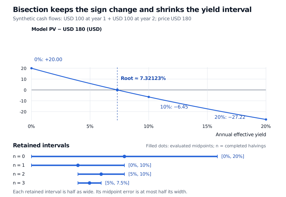
At y=0, the model is USD 20 too expensive. At y=0.20, the residual is −245/9, approximately USD −27.22. The function is continuous throughout [0,0.20], so the intermediate value theorem guarantees at least one zero between those rates. Here it is also strictly decreasing:
f′(y)=−(1+y)2100−(1+y)3200<0for y>−1.
That extra fact establishes uniqueness. Bisection itself does not require monotonicity, and a sign-changing interval alone does not establish uniqueness.
Evaluate the midpoint. If its residual is negative, the rate is too high in this example; retain the left half. If positive, retain the right half. More generally, retain whichever half still has opposite endpoint signs. An exactly verified zero can end the search immediately.
Completed halvings n
Current interval for y
Midpoint mn
Midpoint residual, USD
0
[0,0.20]
0.10
−6.44628
1
[0,0.10]
0.05
5.94104
2
[0.05,0.10]
0.075
−0.44348
3
[0.05,0.075]
0.0625
2.69896
A midpoint can move away from the root on the next step. What reliably improves is the interval bound, not necessarily the realised error of every successive midpoint.
Synthetic two-payment price residual decreases from plus USD 20 at zero yield to minus USD 27.22 at 20 percent. Its root is approximately 7.32123 percent. Four interval rows show widths halving from 20 to 10 to 5 to 2.5 percentage points.
Original synthetic valuation diagram. The curve uses annual effective discounting; filled dots mark evaluated midpoints on the interval rows.
For an independent check, put d=1/(1+y). The equation becomes d2+d−1.8=0. Its positive solution gives y≈0.07321228129313, or 7.321228% annually.
The error certificate has an index
Call the initial interval [a0,b0], its width W0=b0−a0, and its midpoint m0. After n retained-half updates, the current interval has width Wn and midpoint mn. In exact arithmetic, provided the sign-changing bracket is maintained,
Wn=2nW0,∣mn−y∗∣≤2Wn=2n+1W0,
where y∗ is the root retained by the process. The interval width and midpoint error bound differ by a factor of two. A convention that calls the first midpoint m1 produces a different-looking exponent; check the indexing before comparing formulas.
For an absolute parameter tolerance ε>0, sufficient completed halvings are
n≥max{0,⌈log2(2εW0)⌉}.
In this example W0=0.20. A target error of one basis point means ε=0.0001 in decimal yield. Ten halvings suffice. The resulting interval is [0.073046875,0.0732421875]; its midpoint is 0.07314453125 and its error bound is 0.00009765625, or 0.9765625 basis points.
Ten halvings are ten interval updates. With the table's convention, evaluating m0 and every midpoint through m10 takes eleven midpoint evaluations, in addition to the initial endpoints. The final midpoint need not be evaluated merely to obtain the geometric bound.
The radius halves each update, giving a linear convergence bound. This predictability costs function evaluations: Newton's method can be much faster near a suitable simple root; Brent's method combines interpolation with bracket safeguards.
What the guarantee needs
Continuity across the whole interval. The function 1/x changes sign between −1 and 1 but has no zero; the interval crosses a pole. Small interval width around a discontinuity is not evidence of a root.
A valid initial bracket. The continuous function x2 has a root at zero but is positive at both −1 and 1. A strict sign-change test cannot initialise bisection there. Failure to find a bracket does not prove that no root exists. Check endpoint zeros separately.
Trustworthy signs and finite evaluations. A rounded value printed as zero may conceal evaluation error. Compare signs directly rather than multiplying very large or very small floating-point residuals; the product can overflow or underflow. If a sign cannot be trusted, the mathematical bracket certificate cannot be claimed.
A realistic stopping rule. In floating-point arithmetic, the midpoint can round to an endpoint, so another update may make no progress. Detect this and report the achieved bracket and precision limit. Use a midpoint calculation that avoids intermediate overflow, and impose an iteration limit.
A small residual and a small parameter error answer different questions. For g(x)=10−12(x−1), the residual at zero is only −10−12 although the root is one full unit away. Scaling the pricing equation changes residual units and tolerances without changing its root. Report the bracket in yield units and the pricing residual in currency units; neither a numerical tolerance nor extra displayed digits measure market or model uncertainty.
The Root-Finding and Numerical Integration lesson develops the bond-yield formulation alongside Newton and quadrature. A public preview is available; the full lesson requires membership.
SciPy: bisect, continuity, sign requirements and absolute/relative parameter tolerances.
SciPy: brentq, bracketed interpolation and bisection safeguards.
John V. Guttag, Introduction to Computation and Programming Using Python: With Application to Understanding Data, 2nd ed., MIT Press, copyright 2016, §3.3, pp. 30–34, for interval-halving search and approximate computation.