Floating-point arithmetic: Definition & Examples

Floating-point arithmetic represents numbers with a finite significand and an exponent, then rounds arithmetic results to available representable values. It is the arithmetic behind most pricing, portfolio and risk calculations. A tiny discrepancy can be an expected consequence of representation; a large discrepancy still needs investigation.

The exponent lets the scale change while keeping a fixed budget of significant digits. That makes floating point useful for scientific calculations spanning many magnitudes. It does not provide exact real-number arithmetic or a fixed number of decimal places.

Why a decimal sum leaves a binary tail

On the usual IEEE 754 binary64 implementation of Python's float, the following is reproducible:

print(0.1 + 0.2)
# 0.30000000000000004
print(0.1 + 0.2 == 0.3)
# False
print(0.1 + 0.2 - 0.3)
# 5.551115123125783e-17

The decimal fraction $1/10$ has a repeating binary expansion. The stored value is exactly

\frac{3602879701896397}{2^{55}},

which is slightly greater than

1/10

. The input 0.2 is also rounded. Their addition is rounded again, producing the representable number immediately above the stored 0.3. Python's short printed representations conceal most of those exact binary fractions. Formatting a result with fewer decimal places changes its display; it does not repair its stored value. See the official Python floating-point tutorial.

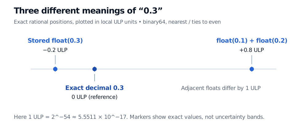
Three exact positions near decimal 0.3: stored float 0.3 is minus 0.2 ULP from the exact decimal, and float 0.1 plus float 0.2 is plus 0.8 ULP. The two stored floats are one ULP apart, equal to 2 to the power minus 54.

Original exact-offset diagram. The reference is the exact decimal fraction $3/10$ ; one local ULP is $2^{-54}$ .

There are two different error comparisons here. Subtracting the stored 0.3 gives exactly

2^{-54}

. Comparing the sum with the exact decimal

3/10

gives

4/(5\cdot2^{54})

, approximately

4.44089\times10^{-17}

. A reported absolute error needs an explicit reference.

The gaps grow with scale

Binary64 uses a sign, an exponent field and a fraction field. A normal finite nonzero value has the form

(-1)^s\left(1+\frac{k}{2^{52}}\right)2^e, \qquad 0\le k<2^{52},\quad -1022\le e\le1023.

The leading

1

is implicit, giving 53 bits of significand precision. Within

[2^e,2^{e+1})

, adjacent positive normal values are

2^{e-52}

apart. A ULP, or unit in the last place, describes that local spacing: it is

2^{-52}

1

and

2^{-51}

2

. At powers of two, spacing below the boundary differs from spacing above it.

With round-to-nearest, ties-to-even arithmetic, an exact midpoint rounds to the candidate whose last significand bit is even. For example,

1+2^{-53}

rounds to

1

. Here we call

2^{-52}

the spacing-based machine epsilon and

u=2^{-53}

the unit roundoff. Authors sometimes call

u

machine epsilon instead; check the convention before using a bound.

For basic operations on stored operands, with a normal finite exact result and no overflow, the usual model is

\operatorname{fl}(x\circ y)=(x\circ y)(1+\delta), \qquad |\delta|\le u, \quad \circ\in\{+,-,\times,\div\}.

This bounds one rounding step. It does not bound an entire pricing algorithm's relative error, nor the error already present in its inputs.

Below the smallest positive normal value,

2^{-1022}

, subnormal values provide a fixed grid with spacing

2^{-1074}

, gradually losing relative precision. Sufficiently small results round to zero. The same uniform relative-error model cannot be applied throughout this region. Overflow, infinities, signed zero and NaN also require explicit handling; the normal-number formula is not the whole format. Oracle's IEEE arithmetic guide documents these formats and rounding rules.

Choose the arithmetic and the acceptance rule separately

For contractual cash amounts, decimal arithmetic or integer minor units can fit the required rounding convention. Constructing Decimal("0.1") preserves the intended decimal input; Decimal(0.1) preserves the already rounded binary input instead. Decimal arithmetic still has finite working precision: division by three does not acquire a terminating expansion. Specify precision, rounding mode and when monetary rounding occurs. The Python decimal documentation explains the controls.

For model outputs, choose comparison tolerances from the scale, units and decision being tested. One common rule is

|a-b|\le\max\!\left(\text{atol},\text{rtol}\max(|a|,|b|)\right).

The absolute tolerance has the units of the output; the relative tolerance is dimensionless. Near zero, an absolute tolerance matters. Neither a universal cent threshold nor the smallest possible machine tolerance is suitable for every price, yield and portfolio weight.

Finally, more digits do not automatically fix catastrophic cancellation or an ill-conditioned problem. Subtracting close computed quantities can expose earlier input errors even when the subtraction itself is exact. Numerical stability concerns how the algorithm propagates these errors. For practical comparisons and debugging, the SelfMadeQuant Testing and Debugging lesson has a public preview; the full lesson requires membership.

Sources

Trefethen, L. N. and Bau, D. III (1997). Numerical Linear Algebra. SIAM. Lecture 13, “Floating Point Arithmetic,” pp. 97–100. Finite representation, spacing and the elementary rounding model.
Python Software Foundation. Floating-Point Arithmetic: Issues and Limitations. Binary fractions and Python representations.
Python Software Foundation. decimal — Decimal fixed-point and floating-point arithmetic. Decimal inputs, contexts and rounding.
Oracle. Numerical Computation Guide, Chapter 2: IEEE Arithmetic. Binary formats, rounding modes and subnormal numbers.

Why a decimal sum leaves a binary tail

The gaps grow with scale

Choose the arithmetic and the acceptance rule separately

Sources

Related terms

Absolute error

Catastrophic cancellation

Numerical stability

Relative error