For a quant developer, the warning sign is a small quantity extracted from large intermediate values: a variance from raw moments, a price increment from two nearby prices, or a hedge residual from large exposures. The formula may be correct in real arithmetic while its evaluation loses the quantity of interest.
The subtraction may be blameless
Suppose the desired quantities are and , but earlier calculations produce and . Even if their subtraction is exact,
For a nonzero true difference, the resulting relative error is
The denominator is the danger. Small errors in the operands need not be small compared with the difference. Their errors might also cancel; a large error is a possibility, not an inevitable consequence of every subtraction.
A small answer that becomes zero
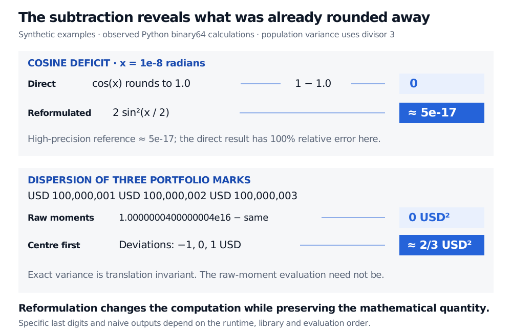
cos(x) rounds to 1.0, so subtracting it from 1 returns zero. That final subtraction is exact for its stored operands; the cosine's small deficit has already disappeared.The identity
provides a better evaluation near zero. It forms the small quantity directly rather than recovering it from a rounded value close to 1.
import math

x = 1e-8
direct = 1 - math.cos(x)
reformulated = 2 * math.sin(x / 2)**2
# direct:       0.0
# reformulated: 5.0000000000000005e-17
The direct result has 100% relative error in this run. Against a 120-digit reference for the actual stored input, the reformulated result has relative error below . The decimal input is itself rounded slightly when stored in binary64; comparing both evaluations against the same stored-input reference isolates their computational error. Specific outputs depend on the mathematical library, precision and evaluation order; a binary64 label alone does not specify every transcendental-function result.
A risk calculation with the same structure
The deviations are USD , USD 0 and USD 1, so USD². Adding a common level to every mark changes the mean but leaves this exact dispersion unchanged.
sum(x*x for x in marks)/3 and mean*mean both evaluate to 1.0000000400000004e16. Subtracting them gives zero. Computing the mean first and then summing the squared deviations gives 0.6666666666666666 USD². The integer marks are all exactly representable in binary64; the raw-moment route loses information in its intermediate arithmetic.This is a numerical demonstration, not an estimate of market volatility from three observations. For real risk data, choose a tested centred, two-pass or online variance algorithm, and consider compensated summation where accumulation error matters. These methods still have finite precision and range limits. They cannot recover mark differences lost during ingestion or fix an inappropriate statistical model. A raw-moment result can even become negative through rounding; silently replacing it with zero hides the diagnostic.
Repair the calculation, and identify what cannot be repaired
As a function of its single input , the cosine deficit has relative condition number
Thus the small nonzero result does not itself make this mathematical problem relatively ill-conditioned near zero. The direct evaluation introduces a fragile intermediate subtraction that the identity avoids. By contrast, if two independently uncertain portfolio values are the original inputs and their difference is the required answer, their uncertainty may already exceed that difference. Algebra cannot manufacture missing input information.
expm1 or log1p for small exponential or logarithmic increments, centre a variance calculation, or increase working precision before the damaging intermediate steps. Verify representative cases against a sufficiently accurate independent reference. At an exact zero, including in the cosine example, relative error is undefined; assess absolute error instead.Sources
- Lloyd N. Trefethen and David Bau III, Numerical Linear Algebra, SIAM, 1997, Lectures 12–14: conditioning, floating-point arithmetic and stability.
- David Goldberg, “What Every Computer Scientist Should Know About Floating-Point Arithmetic”, ACM Computing Surveys, 1991; edited reprint in Oracle's Numerical Computation Guide, especially “Cancellation.”
- David Bindel, Cornell CS 4220: Binary floating point, 2 February 2022, especially the distinction between cancellation and rounding at the subtraction, and the sensitivity of intermediate subproblems.