Find scalar roots with bracketed secant and inverse quadratic interpolation, bisection safeguards, and explicit continuity and stopping checks.
Brent's method
Brent's method is a derivative-free scalar root-finding algorithm that combines a sign-changing bracket with secant and inverse quadratic interpolation, falling back to bisection when an interpolation proposal is unsafe or makes insufficient progress. This Brent–Dekker method is useful when a pricing function can be evaluated reliably but its derivative is expensive or unavailable.
For example, an implied volatility calculation seeks the volatility at which model price minus market price is zero. Brent can search inside a valid volatility bracket without calculating vega. It still needs a continuous residual and trustworthy endpoint signs; the solver cannot create a solution to an inconsistent quote.
Three moves, one safeguard
Bisection proposes the bracket midpoint. A secant proposal instead takes the zero of a straight line through two evaluated points:
s=b−f(b)f(b)−f(a)b−a.
Inverse quadratic interpolation uses three points with distinct function values. It fits a quadratic giving x as a function of the residual t=f(x), then evaluates that quadratic at t=0. Fitting the inverse avoids having to choose between two roots of a quadratic in x.
Brent keeps enough history to choose among these proposals. Its acceptance tests use the current bracket and previous step sizes. An unsuitable interpolation step is replaced by bisection; after evaluating an accepted trial, the endpoints are updated to retain opposite signs unless a root is established. Merely clipping a secant step to the interval does not reproduce these progress safeguards. Brent's own account explains why preventing slow progress matters as well as staying inside the bracket.
The safety result concerns a continuous function on a valid bracket, evaluated with reliable signs. A unique root is not required, although different brackets may select different roots. Fast local behaviour additionally needs a sufficiently smooth function near a simple root, with f′(r)=0. Continuity alone does not promise rapid interpolation or a fixed convergence order for every accepted step.
An interpolation proposal is not a root
Consider the dimensionless test function
f(x)=x3−x−2,[a,b]=[1,2].
Here f(1)=−2 and f(2)=4. Also f′(x)=3x2−1≥2 throughout the bracket, so it contains exactly one root:
r≈1.5213797068045676.
The midpoint is 1.5, with residual −0.125. The line through the two endpoints proposes 4/3, whose residual is −26/27. Neither is the answer.
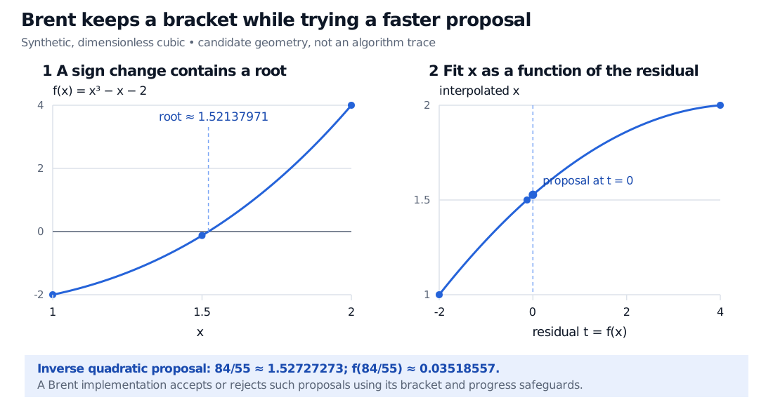
Now take the three evaluated pairs (1,−2), (1.5,−0.125) and (2,4). Their inverse quadratic interpolant proposes
s=5584≈1.52727273,f(s)=1663755854≈0.03518557.
This proposal is close, but its positive residual still matters. If accepted, it would replace the positive endpoint while the negative point at 1.5 preserves a narrower sign-changing bracket. These are illustrative interpolation inputs, not a claimed sequence of Brent iterations. Acceptance and the subsequent trace depend on the implementation and its history.
A cubic changes sign from minus 2 at x=1 to 4 at x=2, with root 1.52137971. An inverse quadratic through x=1, 1.5 and 2 proposes 1.52727273, leaving residual 0.03518557.
Original dimensionless example. The right panel plots the inverse interpolant, not the inverse of the entire cubic. Its proposal must still pass the solver's safeguards and be evaluated in the original function.
What to check at the boundary
A sign reversal across a discontinuity proves nothing about a root: 1/(x−1) has opposite signs at 0 and 2, but no zero. Conversely, (x−1)2 has a root without a sign reversal. Check an endpoint root first, then require continuity across the whole nonzero sign bracket. A singularity, invalid model domain, nonfinite value or noisy evaluation can invalidate the argument.
Choose a parameter tolerance in the units of the unknown. Check the residual separately in price or other output units. A small residual is not automatically a small parameter error: for g(x)=10−12(x−1), the point x=2 has residual 10−12 but root error 1. Root conditioning explains that distinction. With floating-point arithmetic, also check the solver's convergence status, evaluation budget and whether distinct trial points remain representable. A rounded function value of zero alone is not proof of an exact root.
Which Brent routine?
SciPy's brentq implements the bracketed inverse quadratic variant. brenth uses hyperbolic extrapolation instead. They solve the same class of scalar bracketed problems but need not take the same steps. SciPy's brent is a minimizer, a different task. Brent's root solver also differs from Newton–Raphson: it does not require derivatives.
For the finance setup, Root-Finding and Numerical Integration develops a bond-yield residual and basic bisection/Newton methods. The full lesson requires membership; its public preview describes the scope. The cubic above isolates Brent's interpolation logic from pricing conventions.
SciPy, brentq and brenth: algorithm distinctions, bracket requirements and stopping controls; brent documents the separate minimizer.
Tobin A. Driscoll and Richard J. Braun, Fundamentals of Numerical Computation, §4.1, The rootfinding problem: residual, conditioning and simple roots.
John V. Guttag, Introduction to Computation and Programming Using Python: With Application to Understanding Data, second edition, MIT Press, §§3.3 and 3.5: bisection and derivative-based root approximation.