Order of accuracy: Definition & Examples

Order of accuracy describes how an approximation error decreases as a numerical step or mesh spacing shrinks. A method with error proportional to

h^2

is second order in

h

: halving the spacing makes its leading error about one quarter as large. This helps a quant decide whether a finer pricing grid or a smaller Greek bump is buying the expected improvement.

The statement always needs an error measure, a refinement variable and assumptions. “Second order” alone does not specify a price tolerance or guarantee that one implementation is more accurate than another.

The exponent, the constant and the regime

Let $A$ be the exact target, $A_h$ its approximation and $E(h)=\lvert A_h-A\rvert$ . An error bound

E(h)=O(h^p),\qquad h\to0,

means that constants $C$ and $h_0>0$ exist such that $E(h)\le Ch^p$ whenever $0<h<h_0$ , with the problem and other relevant parameters held fixed. The exponent $p>0$ expresses the refinement rate; $C$ controls its scale. This use of Big-O notation concerns approximation error, rather than algorithmic running time.

The familiar prediction

\frac{E(h)}{E(h/2)}\longrightarrow 2^p

needs the stronger leading-term behavior $E(h)=c h^p+o(h^p)$ with $c>0$ . A Big-O upper bound alone does not establish that ratio or an exact order. For a special input the leading coefficient may vanish, producing faster convergence or even an exact answer.

Higher order also does not settle a comparison at one fixed spacing. A large error constant, extra computational work or a grid that is still too coarse can outweigh the asymptotic advantage.

An exact refinement experiment

Consider the dimensionless integral

I=\int_0^1 x^2\,dx=\frac13.

The composite trapezoidal rule uses $n$ equal panels, with $h=1/n$ :

T_n=h\left[\frac{f(0)}2+\sum_{i=1}^{n-1}f(ih)+\frac{f(1)}2\right].

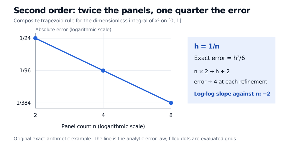
For this quadratic, the line joining the endpoints of each panel lies above the curve. On a panel $[a,a+h]$ , integrating that line and subtracting the exact quadratic area gives $h^3/6$ . There are $n=1/h$ panels, so the total excess is exactly

T_n-I=\frac{h^2}{6}=\frac{1}{6n^2}.

Panels $n$	Spacing $h$	Approximation $T_n$	Absolute error
2	$1/2$	$3/8$	$1/24$
4	$1/4$	$11/32$	$1/96$
8	$1/8$	$43/128$	$1/384$

Each refinement quarters the error. Here that is an exact identity for every positive integer $n$ , rather than an approximate small-step pattern.

Exact trapezoid errors are 1/24, 1/96 and 1/384 at n equal to 2, 4 and 8; each doubling quarters the error.

Original exact-arithmetic example. The line is the analytic error law $h^2/6$ with $h=1/n$ ; filled dots are the evaluated grids. Both axes use logarithmic spacing.

For a general twice continuously differentiable integrand on a fixed interval $[a,b]$ , the bound

\lvert T_n-I\rvert\le \frac{b-a}{12}\max_{x\in[a,b]}\lvert f''(x)\rvert\,h^2

establishes second-order accuracy. The three rows illustrate the result for one function; they do not prove this general theorem. An affine function, for example, is integrated exactly by the trapezoidal rule and has no nonzero error ratio to measure.

What a refinement study can tell you

When an accurate reference is available, estimate an observed order using

p_{\mathrm{obs}}=\frac{\log(E(h)/E(h/2))}{\log 2}.

Without a reference, three nested spacings can give the diagnostic

p_{\mathrm{obs}}\approx \frac{\log\!\left(\lvert A_h-A_{h/2}\rvert/\lvert A_{h/2}-A_{h/4}\rvert\right)}{\log 2},

provided a common nonzero leading error term dominates. In the example, successive differences are $1/32$ and $1/128$ , giving an observed order of 2. Agreement across three grids is useful evidence, but cancellation, coarse-grid effects or an inaccurate reference can make it misleading. Zero differences make this logarithmic diagnostic undefined; they do not establish infinite order.

Which error and which variable?

For time stepping, distinguish local truncation error from global truncation error. Euler's method has a one-step solution defect of $O(h^2)$ when started from the exact solution, yet its global error over a fixed time interval is generally $O(h)$ under suitable smoothness and stability assumptions. Some authors divide the one-step defect by $h$ and call that normalized quantity the local truncation error; under that convention Euler's local truncation error is $O(h)$ . State the convention before comparing exponents.

For a pricing equation with both time and space grids, an error statement such as $O(\Delta t)+O(\Delta x^2)$ describes two different refinement directions. Refining space alone eventually leaves the time error dominant. Boundary approximation and the choice of price or Greek error norm also matter.

An iterative solver's convergence order is a different comparison. An iteration can satisfy

\lvert e_{k+1}\rvert\approx K\lvert e_k\rvert^q

as the iteration index

k

grows. Its exponent

q

relates consecutive iterate errors, whereas mesh accuracy relates error to a spacing

h

. A rapidly converging solver can accurately solve a poorly discretized pricing problem.

A smaller bump eventually stops helping

The stated order normally describes truncation error in exact arithmetic under sufficient smoothness. Floating-point arithmetic, Monte Carlo noise and imperfect inner solves add other error sources. A discontinuity or payoff kink can invalidate the derivatives required by the formal error bound.

For numerical differentiation, shrinking a bump reduces Taylor truncation error while amplifying errors in the price difference after division by that bump. The useful range ends when those other errors dominate. Numerical Differentiation develops forward and central Greek bumps and this trade-off; its full lesson requires membership and has a public preview.

Treat a claimed order as a conditional prediction to check on the quantity you actually report. Hold other error sources sufficiently small, refine systematically and stop interpreting a formal exponent as a promise once the observed errors cease to follow it.

Sources

James Stewart, Single Variable Calculus: Early Transcendentals, 6th edition, Thomson Brooks/Cole, 2008, §7.7, “Approximate Integration”: trapezoidal rule and its second-derivative error bound. The quadratic refinement experiment here is original.
Tobin A. Driscoll and Richard J. Braun, Fundamentals of Numerical Computation, §5.6: Numerical integration: second-order trapezoid convergence and refinement plots.
Driscoll and Braun, §6.2: Euler's method: local-error normalization, global-error assumptions and order of accuracy.

The exponent, the constant and the regime

An exact refinement experiment

What a refinement study can tell you

Which error and which variable?

A smaller bump eventually stops helping

Sources

Related terms

Convergence of a numerical method

Floating-point arithmetic

Integral

Truncation error