Calculus is the mathematics of continuous change and accumulation. It connects two questions that financial models repeatedly ask: how fast is a quantity changing, and how much builds up over an interval? A cash receipt rate measured in dollars per year and the total cash received in dollars are different quantities. Calculus explains how to move between them.
Differential calculus studies local rates through derivatives. Integral calculus studies accumulation through integrals. Their connection, rather than a catalogue of calculation rules, is the starting point.
The same cash stream, read two ways
Suppose a hypothetical contract pays continuously at an increasing rate. Time is measured in years, and the cash receipt rate is
The constant term has units USD per year; the coefficient of has units USD per year squared. The rate begins at USD 20 per year and reaches USD 40 per year at year four. These are assumed payments, not observed market data.
Let be the cash received between time zero and time , with . Ignore interest earned on receipts. Adding the small contributions gives a definite integral:
By year four, the total is
The same answer follows from the trapezoid under the straight rate curve: average rate USD per year, multiplied by four years, gives USD 120. Multiplying the ending rate by four would give USD 160 and overstate receipts: the contract did not pay USD 40 per year throughout.
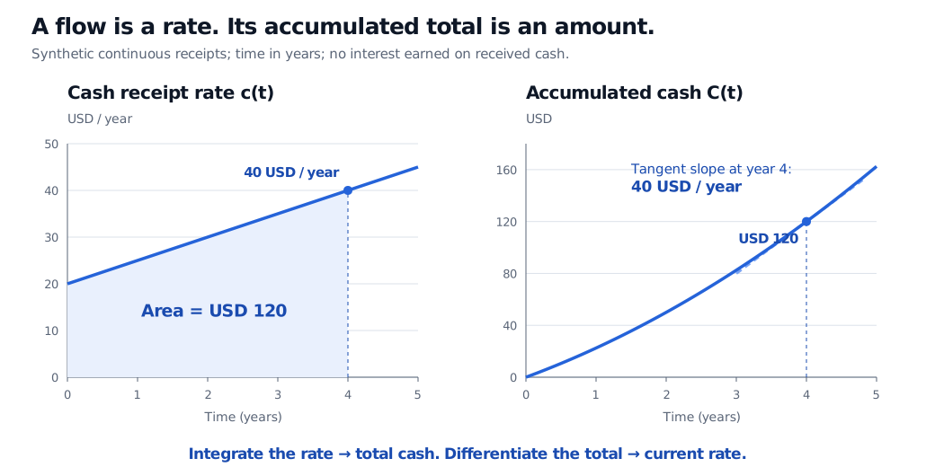
Original hypothetical cash stream. Area under the rate curve measures cash received; slope of the accumulated-cash curve measures the current receipt rate. Received cash earns no interest in this example.
Now read the accumulated total backwards. Its derivative is the limit of its average change over a shrinking time interval:
At year four, USD per year. This says how quickly the total is growing then; it does not say the total equals USD 40. Over the next 0.1 year, a local estimate is USD. The exact extra cash is USD, slightly larger because the receipt rate keeps rising.
The fundamental theorem of calculus makes this connection precise: integrating a continuous rate from a fixed starting point and then differentiating with respect to the upper endpoint recovers that rate. Integrating a derivative recovers the change in the original quantity. A starting balance is additional information; identical receipt rates can accompany different balances.
Which question does the financial model ask?
The variable need not be time. A pricing formula may depend on spot price, interest rates and volatility. A partial derivative measures sensitivity to one input while the others are fixed; option delta is a familiar example. Always name the input and its units. A sensitivity per unit change in a decimal interest rate has a different numerical scale from one per basis point.
Accumulation also depends on what is being added. Our USD 120 is undiscounted cash received, not its present value. For certain receipts and a constant continuously compounded discount rate , measured per year, time-zero value would instead accumulate discounted payments:
At this reduces to USD 120; at it is smaller. If the actual contract pays on discrete dates, use a sum over those dates unless a continuous approximation is justified. Calculus supplies operations on a model; it does not establish that the model fits a contract or predicts markets. For integration in random-path models, see stochastic calculus. The smooth example above supplies no stochastic integration rule.
For a short learning route, Limits and Differentiation develops local sensitivity and its units, then Integration builds accumulated and discounted flows. Both have public previews; the full lessons require membership.
Sources
- James Stewart, Single Variable Calculus: Early Transcendentals, 6th edition (2008), §2.7 (derivatives and rates of change), §5.3 (the fundamental theorem) and §5.4 (net change).
- NIST Digital Library of Mathematical Functions, §1.4, especially derivatives, definite integrals and the fundamental theorem.
- MIT OpenCourseWare, The Second Fundamental Theorem of Calculus, 18.01SC, Fall 2010, explains differentiation of an accumulation function. The contract, calculations and figure here are original.