The beta distribution models bounded proportions or uncertainty about a probability. Read its shapes, endpoint behaviour and beta–binomial update through an order-fill example.
Beta distribution
The beta distribution is a family of continuous probability distributions on the interval from zero to one, controlled by two positive shape parameters. It can describe a bounded proportion, such as a recovery fraction, or uncertainty about an unknown probability, such as an order's chance of filling before a deadline. Those are different modelling uses: a realised fraction is an observation; an unknown probability is a parameter.
Here, write Θ∼Beta(α,β) with α>0 and β>0. Both parameters describe shape. Neither is a rate, a scale, or the market beta of a security.
The density is zero outside the interval. There are no probability atoms at zero or one: the beta law has support [0,1], but P(Θ=0)=P(Θ=1)=0. Even an infinite endpoint density is an integrable limit, not a positive chance of landing exactly there.
A useful alternative is the mean m=α/(α+β) and concentration κ=α+β. Then α=mκ, β=(1−m)κ, and Var(Θ)=m(1−m)/(κ+1). Holding the mean fixed while increasing concentration reduces dispersion. The mean alone does not specify how uncertain the model is.
Updating a fill-probability estimate
Consider a synthetic execution study. Define success as an order filling in full within one second, under a fixed order policy and comparable conditions. Let θ be the common success probability. Before collecting this sample, suppose the desk chooses a prior
Θ∼Beta(2,8).
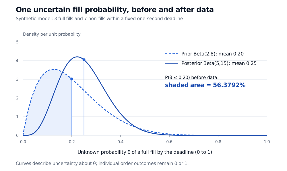
This is an explicit modelling judgement, with prior mean 2/10=0.20, variance 4/275≈0.0145455, and mode 1/8=0.125. A mean of 20% is a summary of the distribution over possible success probabilities; it does not assert that the probability is known to equal 20%.
The next ten orders produce three successes and seven failures. Assume their binary outcomes are conditionally independent, with the same probability θ given Θ=θ. The success count then has a binomial distribution, and its likelihood is proportional to θ3(1−θ)7. Multiplying by the prior gives
π(θ∣data)∝θ2−1(1−θ)8−1θ3(1−θ)7=θ5−1(1−θ)15−1.
The posterior distribution is therefore Beta(5,15). In general, s successes and f failures update the shapes to (α+s,β+f): this is beta–binomial conjugacy. The calculation follows the parameter-update rule in Orloff and Bloom's MIT notes.
Summary of uncertainty about θ
Before data
After data
Distribution
Beta(2,8)
Beta(5,15)
Mean
0.20
0.25
Mode
0.125
2/9≈0.2222
Variance
4/275≈0.0145455
1/112≈0.0089286
The posterior mean lies between the prior mean and the observed success fraction:
205=2010×0.20+2010×103=0.25.
Here α+β supplies the prior's weight in this mean calculation. Calling it a pseudo-count is useful; it need not represent literal earlier orders. Prior data must not be counted again in the new likelihood.
Dashed Beta(2,8) prior and solid Beta(5,15) posterior for an unknown order-fill probability. Mean markers move from 0.20 to 0.25. Prior area below 0.20 is 0.563792384.
Original synthetic model. Three full fills and seven non-fills within the deadline revise the distribution over the shared probability. The shaded area belongs to the prior.
A single future order still has a Bernoulli outcome: success or failure, coded one or zero. Under this model its posterior predictive success probability is E[Θ∣data]=0.25. The beta variance 1/112 measures uncertainty about θ; it is not that order's predictive variance, which is 0.25(1−0.25)=0.1875. Several future orders also share parameter uncertainty, so integrating out Θ does not make their outcomes independent.
The simple update relies on a common, stable probability and the stated likelihood. Changes in liquidity, order size, queue position or routing policy can invalidate that assumption. Conjugacy makes a chosen model easy to update; it does not establish that the model fits execution data. Bayesian Reasoning develops the same update with default probabilities and discusses prior strength. Its public page is a preview; the full lesson requires membership.
Shape and endpoint traps
Beta does not mean bell-shaped. For α,β>1, the density has one interior mode,
θmode=α+β−2α−1.
This formula is conditional on both shapes exceeding one. Differentiating the log density gives (α−1)/θ−(β−1)/(1−θ); outside those conditions, its zero can be a minimum or fail to identify a maximum.
Shape parameters
Density behaviour
α=β=1
Uniform: every point has the same density.
α<1, β<1
U-shaped, with divergent limits at both endpoints and an interior minimum.
α≤1, β≥1, excluding (1,1)
Decreasing; boundary peak toward zero.
α≥1, β≤1, excluding (1,1)
Increasing; boundary peak toward one.
α>1, β>1
One interior maximum at the formula above.
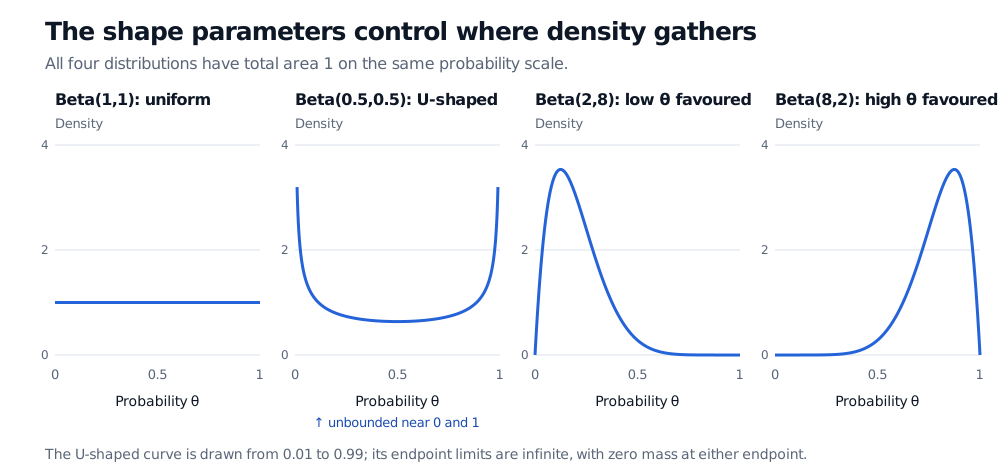
More precisely, the limit near zero is infinite if α<1, finite and equal to β if α=1, and zero if α>1. Swap the parameters to obtain the corresponding limit near one. Boundary peaks describe density limits; they do not create endpoint atoms or probabilities of one.
Four beta densities on the interval zero to one: Beta(1,1) is uniform; Beta(0.5,0.5) is U-shaped with divergent endpoint limits; Beta(2,8) favours small values; Beta(8,2) favours large values.
Original analytic densities. The U-shaped curve is shown only from 0.01 to 0.99; the omitted endpoint limits are infinite, not finite maxima.
Density heights can exceed one. The Beta(2,8) peak is approximately 3.5343, yet its total area remains one. An interval probability comes from integration. For example, its CDF gives
P(Θ≤0.20)=∫00.2072t(1−t)7dt=0.563792384.
If a bounded recovery model needs positive probabilities of exactly zero or exactly full recovery, an ordinary beta density alone cannot supply them. Endpoint masses require a mixture or another explicitly specified model. A beta distribution is also unsuitable for an unbounded variable merely because its observed sample happened to lie between zero and one.
Sources
John A. Rice, Mathematical Statistics and Data Analysis, 3rd ed., §2.2.4 (beta density) and §3.5.2, Example E (Bayesian updating for a binary probability).