A z-test is a hypothesis test that compares a standardized statistic with the standard normal distribution under the null hypothesis, exactly or approximately. For a mean return, it asks how far the observed average is from a specified mean in units of sampling uncertainty. The important question is whether the standard-normal reference is justified, not merely whether the calculation produces a number called .
The clean case: a normal mean with known volatility
Suppose are independent, identically distributed normal observations with unknown mean and known, positive population standard deviation . To test , use the sample mean and its standard error:
Under , exactly. Normal sampling and known make this true even for a small sample; a large sample is not an extra requirement in this model. The denominator is the uncertainty of the average, not the volatility of an individual return. NIST's process-mean guidance distinguishes this known-SD calculation from the more common estimated-SD case.
With denoting the standard-normal cumulative distribution function, the observed statistic gives these p-values:
| Prespecified alternative | p-value |
|---|---|
Choose the alternative before inspecting the result. Switching to a favourable one-sided test afterwards changes the procedure's false-rejection behaviour.
A hypothetical strategy with known risk
For a deliberately idealised example, assume monthly excess returns follow the independent normal model above, with population SD fixed and known to be 2 percentage points. A prespecified sample of 100 months has mean 0.5 percentage points. Test a zero mean against a two-sided alternative:
The two-sided p-value is
Under the zero-mean model, about 1.242% of sample averages are at least this far from zero in either direction. This is not the probability that the zero-mean hypothesis is true. The test rejects at a prespecified 5% level, but fails to reject at 1%.
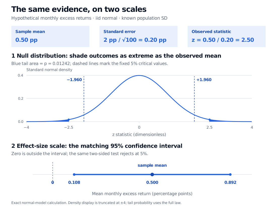
Original hypothetical monthly-return calculation. Blue tails beyond ±2.5 give the observed p-value; dashed lines at approximately ±1.960 mark the fixed 5% rejection thresholds. The lower panel reports the same evidence in percentage points.
The matching 95% confidence interval is
Zero lies outside it, agreeing with the two-sided 5% decision. Here rejection means ; interval endpoints are included, so a null exactly on an endpoint is not rejected. The interval adds the compatible effect sizes that a significance label alone omits.
When “known” is doing too much work
In actual strategy research, population volatility is usually estimated. Replacing with the sample SD changes the exact normal-model statistic to
That calls for Student's t-test, with heavier reference tails. Knowing the numerical value of the sample SD does not make the population SD known. A volatility estimate from an earlier window also carries uncertainty and may describe a different regime. MathWorks' z-test documentation explicitly assumes a normal population and known SD.
The name z-test also covers large-sample procedures whose standardized estimator is only approximately normal. For an iid mean with finite positive variance, the central limit theorem, together with a consistent variance estimate, supports an asymptotic normal reference. There is no universal sample-count threshold that guarantees accurate tail probabilities. Dependence, heavy tails and unstable volatility require attention to the sampling law and the standard-error estimate; having many observations alone does not validate .
For the transition from exact normal pivots to large-sample inference, Confidence Intervals and Hypothesis Testing develops both calculations and their assumptions. Its preview is public; the full lesson requires membership.
Finally, statistical significance does not establish profitability after costs, a stable future edge or robustness to searching many strategies. Those are separate parts of evaluating a return claim.
Sources
- John A. Rice, Mathematical Statistics and Data Analysis, 3rd edition, Duxbury, 2007, §5.3, pp. 183–185; §9.3, pp. 337–338, and §9.4, pp. 339–340: known-variance normal-mean tests and interval inversion.
- NIST/SEMATECH e-Handbook, §7.2.2: Are the data consistent with the assumed process mean?: known versus estimated population SD and normal critical values.
- MathWorks: ztest: normal-population assumptions, statistic, alternative directions and confidence-interval output.