Translate a normal P&L threshold into a standard score, distinguish density from cumulative probability, and read normal tables and 95% cutoffs correctly.
Standard normal distribution
The standard normal distribution is the normal distribution with mean zero and variance one, written Z∼N(0,1). Its standard deviation is also one. It is the common reference that lets a risk analyst translate a loss measured in dollars into a probability: first express the threshold in standard deviations from the mean, then read a cumulative area.
That translation changes coordinates. It does not establish that the original P&L is normally distributed.
It gives the area to the left, ranging from zero to one. For example, ϕ(−2)≈0.053991 is a density height, whereas Φ(−2)≈0.022750 is a probability. For this continuous distribution, P(Z=−2)=0; including or excluding a single endpoint does not change an interval's probability.
These distinguish a lower tail, an upper tail and an interval. A table entry is useful only after deciding which area the question asks for.
From a dollar loss to a standard score
Suppose a hypothetical desk models one trading day's P&L, positive for a profit, as
X∼N(100,2002)in USD.
The mean is USD 100 and the standard deviation is USD 200. The second distribution parameter is variance: 40,000USD2.
What is the model probability of losing at least USD 300? The event is X≤−300. Standardise using
Z=σX−μ,z=200−300−100=−2.
Hence
P(X≤−300)=Φ(−2)≈0.02275013195=2.275013195%.
The threshold is two standard deviations below the mean, even though USD 300 is only 1.5 times the standard deviation. Subtract the mean before dividing. Divide by the standard deviation, not the variance: dollars divided by dollars produce a dimensionless z-score.
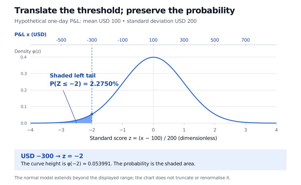
A hypothetical one-day P&L model has mean USD 100 and standard deviation USD 200. USD −300 maps to the dimensionless standard score −2, and the standard-normal area to its left is 2.2750%. The upper axis shows USD and the lower axis shows standard scores.
Original hypothetical normal P&L model. The two horizontal scales locate the same threshold; shading represents probability. The plotted density is that of the standard score, not density per USD. The distribution continues beyond the displayed range.
The calculation is conditional on the specified normal model and horizon. It does not forecast the realised frequency of loss-limit breaches without evidence that this model fits the desk's P&L.
Before using a table, read its heading
Normal tables do not all print the same quantity. At a positive score of 2, these three legitimate conventions give different entries:
Quantity printed
Value, rounded to ten decimal places
Recover the lower tail at −2
Left cumulative area Φ(2)
0.9772498681
1−Φ(2)
Area between zero and two
0.4772498681
0.5−P(0<Z≤2)
Upper tail P(Z>2)
0.0227501319
Use directly by symmetry
The NIST standard-normal table, for example, prints area from zero to the positive score, so its entry at 2.00 is 0.47725. Treating that number as Φ(2) would choose the wrong area. Round the final answer after converting the table convention.
In software, use a survival-function or upper-tail routine for very small upper tails when available. Subtracting a CDF already rounded near one can lose meaningful digits; a displayed zero need not mean mathematical impossibility.
Reading the reference backwards
A quantile function reverses the calculation: for a desired cumulative probability p, find zp=Φ−1(p). For a normal X,
xp=μ+σzp.
The familiar 1.96 is a rounded cutoff:
P(−1.96≤Z≤1.96)=2Φ(1.96)−1≈95.00042%.
The exact central 95% cutoff is Φ−1(0.975)≈1.9599639845. In the desk example, the rounded interval 100±1.96(200) is USD −292 to USD 492. This is a central probability interval for one day's P&L under known model parameters. A confidence interval for an unknown mean answers a different question and uses the sampling variability of an estimator.
Finally, any variable with finite mean and positive finite variance can be centred and scaled to mean zero and variance one. That alone does not make it standard normal. A non-normal distribution retains its shape under this transformation. If the mean or volatility is estimated, its uncertainty also remains; replacing them with estimates does not make a new observation an exact standard-normal draw.
For a guided continuation, Normal Distribution in the Mathematics Primer develops standardisation and financial tail probabilities. The full lesson is available with a free signed-in account; the public page provides a preview.
Sources
Bertsekas, D. P., and Tsitsiklis, J. N. (2008). Introduction to Probability, 2nd ed., §3.3, “Normal Random Variables,” pp. 154–157: the standard normal, symmetry, its table and standardisation.