Volatility of volatility measures uncertainty in volatility itself. Read Heston’s variance coefficient, local volatility changes and time units correctly.
Volatility of volatility
Volatility of volatility, or vol of vol, describes the size of random fluctuations in volatility itself. In a stochastic-volatility model, it controls an additional source of uncertainty beyond the asset's return volatility. Two models can start with the same 20% stock volatility and produce different option prices because their future volatility can move by different amounts.
The phrase needs a model and a convention. A coefficient in a variance equation, an absolute volatility-change standard deviation, and a relative volatility-change standard deviation are different quantities. A bare “vol of vol = 0.30” does not identify all three.
Read the equation before the number
In the Heston model, the stock's instantaneous return volatility is σt=vt, where the instantaneous variance rate follows
dvt=κ(θ−vt)dt+ξvtdWtv.
Here Wtv is Brownian motion, κ controls mean reversion, θ is the long-run variance level, and ξ≥0 is conventionally called vol of vol. The stock and variance Brownian shocks may be correlated; this is separate from the magnitude ξ.
The variance's diffusion coefficient is ξvt, not ξ alone. Conditional on the current state and for a small interval Δt,
SD(vt+Δt−vt∣vt)≈ξvtΔt.
These are leading local diffusion scales. They do not make the exact finite-horizon Heston variance transition Gaussian, and a negative draw from a naive Gaussian approximation is not a valid negative variance state.
Use a synthetic model with time in years, κ=2, θ=0.04, current variance vt=0.04, and ξ=0.30. The current annualised volatility is 0.04=0.20, quoted as 20%. Define one model trading day as Δt=1/252 year.
The local standard deviation of the variance-rate increment is
0.30×0.20×1/252≈0.003780.
To express uncertainty in volatility, apply the local square-root sensitivity dv/dv=1/(2v):
SD(σt+Δt−σt∣vt)≈2×0.200.0037796447…≈0.009449.
That is about 0.945 volatility percentage points, an absolute change in the annualised quote. It is neither 30 percentage points nor the stock's 20% annualised return volatility. The variance drift is zero at this particular state because vt=θ; the square root still introduces a drift correction for volatility.
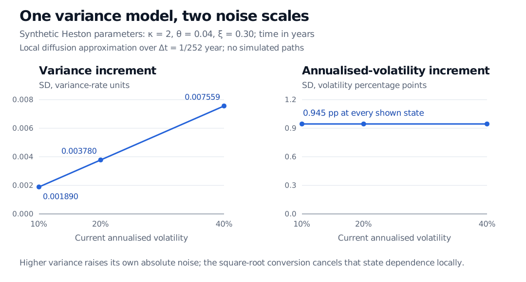
With synthetic Heston vol of vol 0.30 and a 1/252-year interval, current annualised volatilities of 10%, 20% and 40% have local variance-increment standard deviations 0.001890, 0.003780 and 0.007559. The local annualised-volatility-increment standard deviation stays at about 0.945 percentage points.
Original analytic comparison, with time in years. Both panels use the same synthetic Heston parameters; the vertical units differ. The volatility panel uses the local square-root transformation, not exact finite-horizon transition intervals or simulated paths.
Itô's lemma makes the distinction precise. Away from vt=0,
dσt=(2vtκ(θ−vt)−8vtξ2)dt+2ξdWtv.
The absolute volatility diffusion coefficient is ξ/2, here 0.15. Its relative diffusion coefficient, obtained by dividing by σt, is ξ/(2vt) and varies with the state. Thus, even within one model, “vol of vol” can refer to different numerical objects unless the equation is supplied.
With dimensionless returns and years as the time unit, v has units year−1, σ has units year−1/2, κ and ξ have units year−1, and Brownian increments have units year1/2. Changing the time unit requires changing the coefficients and the variance-rate convention together. The parameter 0.30 cannot simply be relabelled as a daily coefficient.
What the parameter changes—and what it does not
A larger ξ increases the local variance uncertainty at a fixed state. Through the distribution of future variance and its interaction with stock returns, it also affects option prices and the implied-volatility smile. The effect depends on correlation, mean reversion, maturity and strike; it is not a rule that every option becomes more expensive. Nor is ξ an implied volatility read directly from one option quote.
If ξ=0, variance evolves deterministically. It is constant only when its initial value equals θ; otherwise it still mean-reverts. Zero vol of vol therefore does not, by itself, mean zero stock volatility.
The numerical example also satisfies the Feller condition: 2κθ=0.16>ξ2=0.09, so a positive initial CIR variance does not reach zero. The displayed volatility transformation is valid in that positive region. If the boundary is attainable, its singular drift needs appropriate boundary treatment; the local square-root calculation should not be extrapolated through zero.
Jim Gatheral, The Volatility Surface: A Practitioner's Guide (Wiley, 2006), Chapter 1, equations (1.1)–(1.2), and Chapter 2, “The Process,” pp. 15–16, equations (2.1)–(2.2) — stochastic variance, parameter conventions and the Heston square-root process. The local noise calculations and figure above are original synthetic examples.