Stochastic volatility: Definition & Examples

Stochastic volatility means that an asset's instantaneous volatility evolves randomly through time. The model treats the future intensity of price fluctuations as uncertain, alongside the future price itself. For an options desk, this adds a risk that a constant-volatility model suppresses: tomorrow's volatility state can change the value of a position even when spot barely moves.

Start with volatility and Brownian motion. A stochastic differential equation then describes how today's state responds to drift and new random shocks.

Random price, random variance

In the constant-volatility Black–Scholes model, the stock price is random but its volatility parameter is fixed. Replacing that constant by a known calendar schedule

\sigma(t)

changes the amount of uncertainty over time, but the schedule itself remains deterministic.

A stochastic-volatility model gives volatility, or often variance, its own random dynamics. In the Heston model, the pricing equations with constant risk-free rate

r

and continuous dividend yield

q

are

\begin{aligned} \frac{dS_t}{S_t} &= (r-q)\,dt+\sqrt{v_t}\,dW_t^S,\\ dv_t &= \kappa(\theta-v_t)\,dt+\eta\sqrt{v_t}\,dW_t^v,\\ dW_t^S\,dW_t^v &= \rho\,dt. \end{aligned}

These equations are under the risk-neutral measure

\mathbb{Q}

. The two Brownian shocks have instantaneous correlation

\rho

. Gatheral develops this square-root variance specification in Chapter 2 of The Volatility Surface; Heston's original paper explains the role of correlation in return skewness and option pricing.

The distinction between $v_t$ and $\sqrt{v_t}$ matters:

Quantity	What it means
$v_t$	Instantaneous variance rate: decimal return squared per year when time is in years
$\sqrt{v_t}$	Instantaneous volatility: decimal return per square root of a year
$\theta$	Long-run mean variance, not long-run mean volatility
$\kappa>0$	Speed of variance mean reversion, per year
$\eta>0$	Scale of the variance diffusion, conventionally called “vol of vol”
$\rho\in[-1,1]$	Correlation between spot-return and variance shocks

For example, $v_t=0.04$ corresponds to 20% annualised instantaneous volatility, not 4%. Nor is $v_t$ the variance of the price in currency units: the stock's diffusion coefficient is $S_t\sqrt{v_t}$ .

With $\rho<0$ , a negative spot shock tends to accompany a positive variance shock. This is a probabilistic relationship between shocks. It does not mean every fall in the stock must raise volatility; the variance drift and the other component of its random shock still matter.

A six-month variance forecast inside the model

Suppose a hypothetical pricing model uses

v_0=0.04,\qquad \kappa=2,\qquad \theta=0.09,\qquad \eta=0.30,\qquad \rho=-0.70,

with time in years and returns in decimals. These are illustrative parameters, not estimates from a traded asset.

Mean reversion pulls variance toward

0.09

, but individual paths wander around that pull. Taking the conditional expectation of the variance equation gives the moment equation

m'(t)=\kappa(\theta-m(t))

, with

m(0)=v_0

. Hence

\mathbb{E}^{\mathbb{Q}}[v_T\mid v_0] =\theta+(v_0-\theta)e^{-\kappa T}.

At $T=0.5$ years,

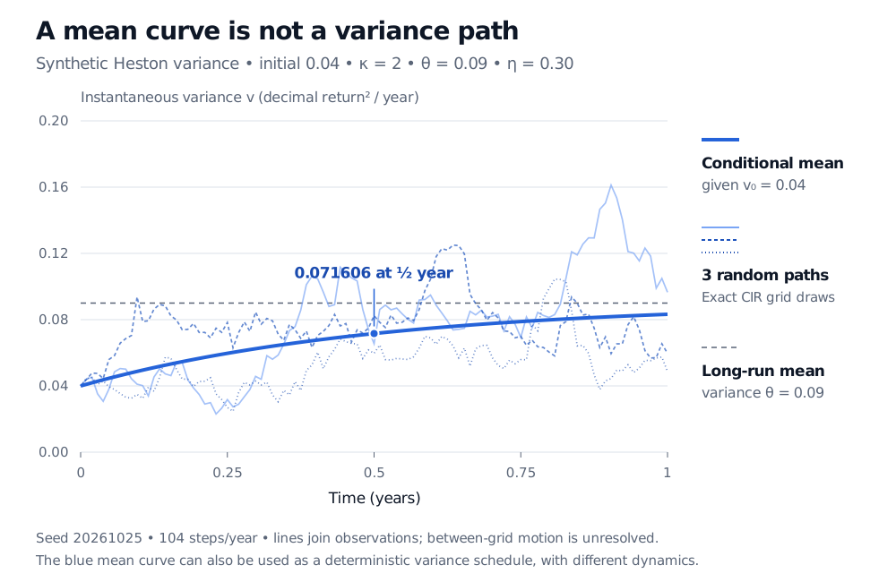
\mathbb{E}^{\mathbb{Q}}[v_{0.5}\mid v_0=0.04] =0.09-0.05e^{-1} \approx0.071606.

Variance starts below its long-run mean, so its conditional mean rises. That statement does not predict a monotone rise on a particular path. The initial state is fixed here; the process is not started in its stationary distribution.

Three synthetic Heston variance paths start at 0.04 and fluctuate around a rising conditional mean. The mean reaches 0.071606 at half a year and tends toward the long-run mean variance 0.09. The vertical axis is decimal return squared per year; the horizontal axis is years.

Original synthetic example. Three seeded paths use exact CIR transition draws at 104 steps per year; joining the observations does not resolve motion between them. The solid blue curve is the analytic conditional mean, not an average of these three paths. Only the variance process is simulated.

Taking the square root gives

\sqrt{\mathbb{E}^{\mathbb{Q}}[v_{0.5}\mid v_0]} \approx26.76\%.

This is a root-mean-variance quantity. It is not the expected instantaneous volatility. The square-root function is concave, so Jensen's inequality gives

\mathbb{E}^{\mathbb{Q}}[\sqrt{v_T}\mid v_0] \leq\sqrt{\mathbb{E}^{\mathbb{Q}}[v_T\mid v_0]}.

For non-degenerate future variance, the inequality is strict. Likewise,

\sqrt{\theta}=30\%

is the square root of the long-run mean variance; it is not the stationary mean volatility. Neither number is automatically the implied volatility of a six-month option: that comes from an option price, with its strike and full model dynamics.

What this changes for pricing and hedging

An option's value now depends on both spot and the variance state. A hedge that offsets a small spot move can still lose when variance changes. With two independent sources of Brownian uncertainty and only stock and cash to trade, spot delta alone generally cannot remove the extra variance risk.

The volatility smile provides information about pricing dynamics, but it does not hand over a unique physical forecast. Parameters fitted to option prices belong to the chosen pricing measure. Parameters estimated from historical observations describe dynamics under the physical measure

\mathbb{P}

. A volatility-risk premium can make the variance drift differ between them. Simply replacing a historical stock drift by

r-q

does not justify carrying the historical variance drift across unchanged.

Also keep three modelling choices separate:

A deterministic time schedule $\sigma(t)$ is known in advance.
Local volatility $\sigma(S_t,t)$ is a specified function of spot and time. Its realised value is random because spot is random, but it has no separate variance state.
Stochastic volatility introduces a random volatility or variance factor, as Heston does above. Heston is one member of this family, not its definition.

Using the blue conditional-mean curve as a deterministic variance schedule would preserve that curve, but discard the uncertainty around it. Equal expected variance curves do not imply equal option prices, forward-smile behaviour or hedge performance.

Positive theory does not make Euler steps positive

For the exact square-root variance process, positive parameters and $v_0>0$ give non-negative variance. The Feller condition

2\kappa\theta\geq\eta^2

makes zero unattainable. Here $2(2)(0.09)=0.36$ , whereas $0.30^2=0.09$ , so the condition holds. If it fails, the exact process can reach zero; failure does not authorize negative variance.

An ordinary Euler discretisation has a different issue:

v_{n+1}=v_n+\kappa(\theta-v_n)\Delta t +\eta\sqrt{v_n\Delta t}\,Z,\qquad Z\sim\mathcal{N}(0,1).

Because the normal shock is unbounded, an Euler step can be negative even when the Feller condition holds. With the same initial state, a deliberately coarse $\Delta t=0.5$ and $Z=-3$ , the update is about $-0.037279$ . That is an artefact of the scheme, not a valid state of the exact model.

Truncation schemes, other specialised discretisations and exact transition sampling address this in different ways. Their treatment of the variance boundary and their pricing bias require checks. Exact sampling of the variance at observation dates alone does not provide an exact joint simulation of the stock and its integrated variance. Gatheral's Chapter 2 makes this theoretical-versus-numerical distinction explicit.

For the next step, Stochastic Volatility and the Heston Model develops parameter interpretation, pricing routes and simulation. The public page is a preview; the full lesson requires membership.

Sources

Jim Gatheral, The Volatility Surface: A Practitioner's Guide (Wiley, 2006), Chapter 2, “The Heston Model,” pp. 15–16 and 21–23: square-root variance dynamics, correlation and simulation methods.
Steven L. Heston, “A Closed-Form Solution for Options with Stochastic Volatility with Applications to Bond and Currency Options”, The Review of Financial Studies 6(2), 1993, pp. 327–343, doi:10.1093/rfs/6.2.327.

Random price, random variance

A six-month variance forecast inside the model

What this changes for pricing and hedging

Positive theory does not make Euler steps positive

Sources

Related terms

Black-Scholes model

Brownian motion

Conditional expectation

Implied volatility

Mean reversion

Stochastic differential equation

Volatility

Volatility smile