A sequential probability ratio test stops when evidence crosses a boundary. Follow a Bernoulli example, first-stop semantics and exact versus nominal error rates.
Sequential probability ratio test
A sequential probability ratio test (SPRT) compares two specified statistical models as observations arrive, stopping the first time their likelihood ratio crosses an upper or lower boundary. It can decide earlier than a fixed sample design when evidence accumulates quickly. For a quant monitoring a binary outcome stream, the useful change is that when to stop is part of the test, rather than an informal decision made after inspecting results.
The classical construction below tests two simple hypotheses: each fixes the entire distribution. It does not automatically answer an open-ended question such as whether a strategy has any positive edge. Perlman's sequential-testing notes, §19.1 introduce this model comparison.
Evidence has a direction—and a stopping rule
Let X1,X2,… be independent, identically distributed observations with probability mass function or density f0 under the null hypothesis and f1 under the alternative hypothesis. Define the likelihood ratio with the alternative in the numerator:
Large values favour H1; small values favour H0. The log form accumulates evidence by addition. A source using L0/L1 reverses the directions, so check the numerator before copying a decision rule.
Write α for the nominal Type I error target and β for the nominal Type II error target. Wald's conventional boundaries are
A=α1−β,B=1−αβ,0<B<1<A.
After each observation, apply the following rule only if the test has not already stopped:
Current evidence
Action
Λn≥A, or Zn≥logA
Stop and choose H1
Λn≤B, or Zn≤logB
Stop and choose H0
B<Λn<A
Continue
Here “choose” means make the test's terminal decision between these two models; it does not prove that either model is literally true. These are approximate error-calibration formulas: an observation can carry the statistic past a boundary rather than exactly onto it. Stefan and coauthors, “Stopping rules and error rate control”, discuss this overshoot and the distinction between nominal and effective errors.
Eight successes, then stop
Consider a fictional monitoring experiment in which each observation records whether an execution meets a predeclared criterion: Xi=1 for success and Xi=0 otherwise. Assume independent Bernoulli outcomes with one constant success probability throughout the experiment. Compare
H0:p=0.4withH1:p=0.6,α=β=0.05.
The parameters are illustrative model values, not execution-quality targets. With sn successes and n−sn failures, the Bernoulli likelihood gives
Each success adds log(1.5)≈0.405465; each failure subtracts the same amount. This follows directly from the binary likelihood described in Penn State's likelihood-methods notes, using the reciprocal ratio convention here.
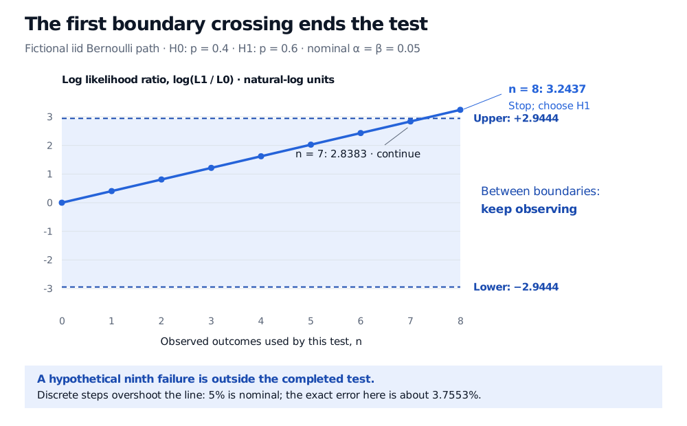
The boundaries are A=19 and B=1/19, or approximately ±2.944439 on the log scale. Suppose the first eight outcomes are all successes:
Observation
Log likelihood ratio
Decision
7
7log(1.5)=2.838256
Continue
8
8log(1.5)=3.243721
Stop; choose H1
At the stop, Λ8=1.58=25.62890625, beyond the threshold of 19. A hypothetical ninth failure is not processed by this completed test. Recomputing a running statistic after the stop and withdrawing the decision would define a different procedure.
Fictional iid Bernoulli SPRT comparing p 0.4 with p 0.6: seven successes give log likelihood ratio 2.838256 below the upper boundary 2.944439; eight give 3.243721 and stop the test. The lower boundary is minus 2.944439. Later observations are excluded.
Original model calculation. Each success adds log 1.5; the first crossing occurs at observation 8. The continuation region lies between the two dashed boundaries.
What “nominal 5%” means in this example
We can calculate the exact errors here without simulation. Let Dn=2sn−n, successes minus failures. Because 7log(1.5)<log19<8log(1.5), stopping occurs when Dn first hits +8 or −8.
Under H0, let h(k) be the probability of eventually hitting +8 before −8, starting at D=k. It obeys
h(k)=0.4h(k+1)+0.6h(k−1),h(−8)=0,h(8)=1.
Solving this recurrence gives the false-rejection probability from D0=0:
h(0)=1−1.5161−1.58=1+1.581=6817256≈3.7553%.
Swapping success and failure gives the same probability of choosing H0 under H1. Both exact errors are therefore about 3.7553% for this infinite-horizon, iid design with no truncation. The nominal 5% inputs did not produce exact 5% errors. This calculation is specific to these Bernoulli models and boundaries.
Applying the idea to financial data
A live success stream can contain serial dependence, changing market conditions and delayed outcomes. Then the iid likelihood above is misspecified. A dependent-data model needs the correct joint or conditional likelihood; simply multiplying marginal Bernoulli probabilities does not fix the problem. Unknown nuisance parameters, composite alternatives, a maximum sample size or a changed observation schedule also require a design whose operating characteristics account for those choices.
Repeatedly checking an ordinary fixed sample hypothesis test and stopping when it rejects does not turn it into an SPRT. Likewise, the terminal likelihood ratio is neither a p-value nor a posterior probability; posterior odds additionally need prior odds. The assumptions and stopping rule jointly determine what the decision can support.
For the fixed sample foundations, The Hypothesis Testing Framework explains simple versus composite hypotheses and both error types. Its preview is public; the full lesson requires membership.
Penn State STAT 509, §9.2: Likelihood Methods: binary likelihoods and sequential boundary comparisons. Its ratio places the null in the numerator; this article explicitly uses the alternative in the numerator.