A return time measures a revisit to the starting state. See why self-loops count, why transition probabilities are not first-return probabilities, and when the mean can be infinite.
Return time
A return time is the elapsed time until a process revisits a state where it started. For a discrete-time Markov chain, the standard first return time excludes the initial observation but includes the very next observation, even if the chain has stayed in the same state. This convention matters when a quant translates a regime's long-run frequency into an average wait: consecutive Calm days count as consecutive visits, rather than as a single Calm episode.
Let X0=i. Write
τi+=inf{n≥1:Xn=i},inf∅=∞.
The superscript + stresses that time zero is excluded. By contrast, a first-passage time defined using n≥0 is zero when the process already starts at its target. A return time is a stopping time: whether the return has occurred by today is known from observations through today.
A market can return without having left
Consider a synthetic daily regime model with states Calm (C) and Stress (S). Rows and columns of its transition matrix follow that order:
P=(0.80.30.20.7),X0=C.
These probabilities illustrate the mathematics; they are not estimated market transition rates. Tomorrow is Calm with probability 0.8, so PC(τC+=1)=0.8. A self-loop counts as a return.
For a first return on day k≥2, the chain must leave for Stress on day one, remain there until day k−1, and enter Calm on day k:
PC(τC+=k)=0.2(0.7)k−20.3,k≥2.
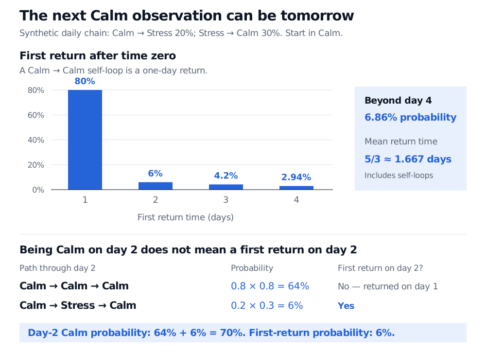
In particular, a first return on day two has probability 0.2×0.3=0.06. But the probability of simply being Calm on day two is
(P2)CC=0.82+0.2×0.3=0.70.
The additional 0.64 comes from Calm → Calm → Calm paths, which already returned on day one. Powers of the transition matrix count endpoint visits, including paths with earlier returns; they do not directly give the first-return distribution.
Exact synthetic daily return-time law from Calm: probabilities on days 1 to 4 are 80%, 6%, 4.2% and 2.94%, with 6.86% beyond day 4. Mean return time is 5/3 days. The two paths ending in Calm on day 2 have probabilities 64% and 6%; only the second first returns on day 2.
Original exact calculation for the stated synthetic daily chain. The bars show first returns; the path comparison separates a day-two endpoint from a day-two first return.
If the risk question is “How long until Calm returns after we have entered Stress?”, start the clock in Stress and measure its first passage to Calm. If the clock starts today but must first wait for departure, it also includes the initial Calm spell. Both differ from τC+. Specify the event and clock origin before interpreting a reported recovery time.
A short average with a long tail
Starting in Stress, let gS be the expected days to reach Calm. First-step conditioning gives gS=1+0.7gS, hence gS=10/3 days. Starting in Calm, the next observation always consumes one day; only the Stress branch adds a further wait:
EC[τC+]=1+0.2gS=35≈1.667 days.
The small mean reflects the many one-day returns. It does not promise a quick recovery conditional on entering Stress, nor guarantee a return by any finite deadline.
There is another way to obtain the mean. For an irreducible positive-recurrent, time-homogeneous chain with stationary distributionπ,
Ei[τi+]=πi1.
Here the stationary flow balance 0.2πC=0.3πS, together with πC+πS=1, gives πC=0.6. Its reciprocal is 5/3 days, agreeing with the first-step calculation. The identity concerns the spacing between visits to a state; interpreting it as spacing between distinct regime episodes would discard the self-loops that the formula counts. Aperiodicity is not required for this mean-return identity.
Returning eventually does not ensure a finite mean
A recurrent state has return probability one. It is positive recurrent when the mean return time is finite and null recurrent when that mean is infinite. The symmetric random walk on all integers is the classic null-recurrent example: it returns to its starting integer almost surely, yet its expected return time is infinite. An irreducible null-recurrent chain has no stationary probability distribution; assigning zero probability to every integer cannot produce one.
For a transient state, there is positive probability of never returning, recorded as τi+=∞. Its unconditional extended mean is therefore infinite, even if a conditional mean among returning paths is finite. A return-time histogram that silently drops nonreturning paths answers a different question.
In a time-homogeneous chain started at a recurrent state, successive inter-return durations are i.i.d. by the strong Markov property. They therefore supply a renewal process. Finite mean is an extra condition needed for the usual positive long-run visit rate.
Sources
Richard Durrett, Essentials of Stochastic Processes, third edition (Springer, 2016), §1.7, Theorem 1.21 and the cycle argument; §1.11, Theorem 1.30: return-time identity and the distinction between recurrence and positive recurrence.
Richard Weber, Markov Chains, University of Cambridge notes (October 2011), §§5.1–5.2 and 8.2, Theorem 9.1 and Example 9.2: positive-time convention, recurrence classification and the null-recurrent integer walk.