A transient Markov-chain state has a positive chance of never returning. Repeated visits are possible, but their expected total is finite.
Transient state
A transient state of a time-homogeneous, discrete-time Markov chain is a state that, when started there, has a positive probability of never being visited again after time zero. The chain visits it only finitely many times, almost surely; its expected total number of visits is also finite.
In a regime model, transience can encode a phase the system eventually leaves behind. This matters when using long-run regime weights to assess risk: a state with no long-run weight can still dominate the next few observations. Classification is a statement about the chosen model, not evidence that an observed market regime can never reappear.
Return is allowed
Let the first return time to state i be
τi+=inf{n≥1:Xn=i},inf∅=∞,
and write fii=Pi(τi+<∞), where the subscript means X0=i. Transience means fii<1; a recurrent state has fii=1. A self-transition at the next step counts as a return, even if the chain has not left the state.
“Transient” does not mean “visited at most once.” It allows repeated visits, including departures followed by returns. For example, a state may lead to a second state that sometimes sends the chain back and sometimes sends it into a permanent exit. What matters is that continued returns eventually stop with probability one.
A phase that can linger
Suppose a hypothetical model has an initial regime T and two enduring regimes C1,C2. One step is one day. In that order, the row transition matrix is
P=1/2001/43/41/21/41/41/2,X0=T.
The probabilities are stipulated, not fitted to market data. Each day in T, the model remains there with probability 1/2. Otherwise it enters the closed communicating class{C1,C2}. Once it leaves T, there is no route back. That last feature belongs to this example; it is not required for transience in general.
Starting at T, the only possible first return is tomorrow's self-transition. Hence fTT=1/2. Yet the chain can remain in T for any finite number of days with positive probability. There is no predetermined departure date.
The chance of being in T after n days is
PT(Xn=T)=(21)n.
After four days it is 1/16=6.25%. The probability of staying there forever is the limit of these probabilities, zero.
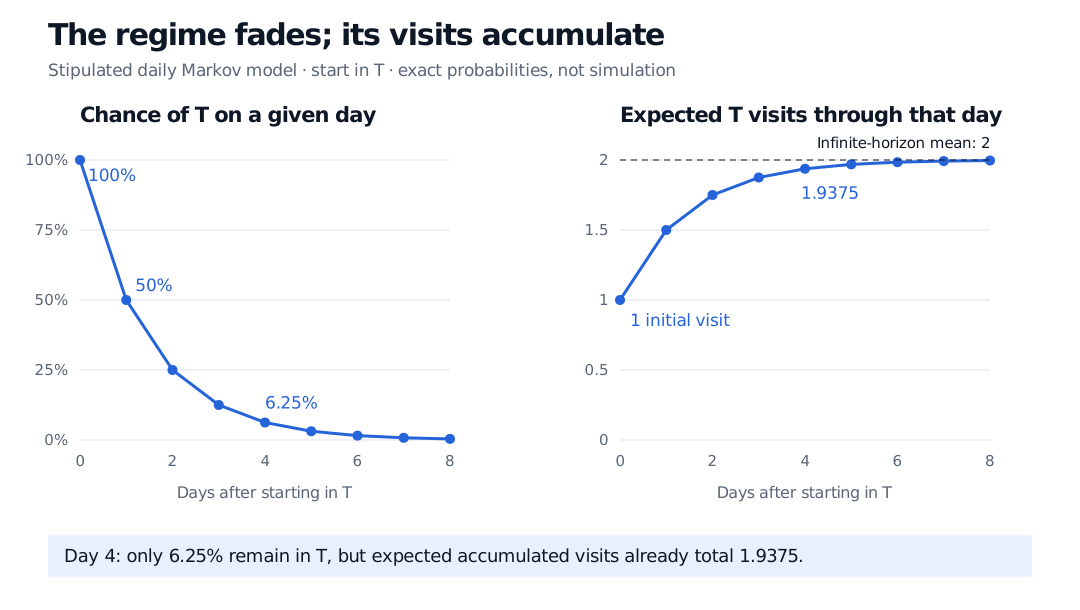
Starting in transient regime T, its day-n probability is 2 to the power minus n: 100% initially, 50% after one day and 6.25% after four. Expected visits including day zero rise from 1 to 1.9375 through day four and approach 2.
Exact daily model starting in T. Filled dots mark integer days; joining lines are guides. The left panel is a probability at one time; the right adds expected visits from day 0 through that time.
Counting the visits
For a general transient state, let Vi=∑n=0∞1{Xn=i} count all visits, including the initial one. Each successful return restarts the same return question. Thus
Pi(Vi=k)=(1−fii)fiik−1,k=1,2,…,
and
Ei[Vi]=1−fii1=n=0∑∞(Pn)ii<∞.
The expected number of returns, excluding time zero, is instead fii/(1−fii). These two counts differ by one. Durrett's §1.3 derives the visit-count criterion; Cambridge's notes, §5 give the equivalent summability and return-probability tests.
In our model, PT(VT=k)=2−k and ET[VT]=2. That mean is not a maximum: the probability of at least four visits is 1/8. Through day four, the expected accumulated count is already 1+1/2+1/4+1/8+1/16=1.9375. A quickly shrinking current probability and meaningful cumulative exposure can coexist.
The states C1,C2 are recurrent because they form a finite closed communicating class. Neither is an absorbing state: the model continues moving between them. Its stationary distribution is (0,2/3,1/3). The zero weight on T captures its long-run disappearance, while the initial distribution puts probability one there. A risk calculation for the coming days should retain that initial condition.