A stationary distribution balances Markov-chain probability flows. A regime example separates invariant weights, finite-horizon forecasts and long-run occupation.
Stationary distribution
A stationary distribution, also called an invariant distribution, is a probability law that a Markov chain leaves unchanged after one transition. If the chain starts with this law, its state has the same distribution at every later date.
In a regime model, stationary weights can describe the model's long-run allocation of time across market conditions. They answer a different question from “given that today is calm, what is the probability of stress tomorrow?” Confusing the two can replace a relevant short-horizon risk forecast with an equilibrium average.
Probability that balances while states keep changing
Consider a hypothetical daily chain with states Calm and Stress. Its probabilities are stipulated for teaching, not fitted to market data. Use row probability vectors and the transition matrix
P=(0.80.30.20.7).
A Calm day is followed by Stress with probability 0.2; a Stress day is followed by Calm with probability 0.3. A stationary row vector π=(πC,πS) must satisfy
πP=π,πC+πS=1,πC,πS≥0.
The Calm equation is 0.8πC+0.3πS=πC, or 0.2πC=0.3πS. Together with normalisation, this gives
π=(0.6,0.4).
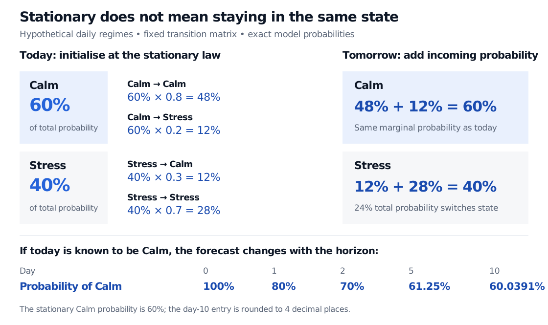
The equation balances probability flows, rather than freezing the state. At stationary initialisation, the joint probability of Calm today and Stress tomorrow is 0.6×0.2=0.12. The reverse flow is 0.4×0.3=0.12. These cancel, leaving each state's total probability unchanged. Nevertheless, the probability of a switch on any given day is 0.12+0.12=0.24.
Stationary initial probabilities of 60% Calm and 40% Stress create one-day flows of 48% Calm to Calm, 12% Calm to Stress, 12% Stress to Calm and 28% Stress to Stress. Incoming totals remain 60% and 40%, although 24% switches state. Starting entirely Calm instead gives Calm probabilities 100%, 80%, 70%, 61.25% and approximately 60.0391% at days 0, 1, 2, 5 and 10.
Exact probabilities for a hypothetical daily model. Stationary initialisation preserves the marginal weights; knowing today's state produces a horizon-dependent forecast. The day-10 percentage is rounded.
Balancing every pair separately is called detailed balance. It works here, but general stationary chains can have circulating flows: stationarity requires total inflow to equal total outflow at each state, without requiring cancellation along every pair. The Detailed Balance and Time Reversibility lesson proves why pairwise balance is sufficient. The full lesson requires membership; a public preview is available.
Start in equilibrium, or approach it
Let qn be the state distribution after n days. The Chapman–Kolmogorov equations give qn=q0Pn.
If q0=π, then qn=π for every n: there is no waiting period before the distribution becomes stationary. With the fixed homogeneous transition rule, the resulting state process is also stationary under shifts of the observation dates. Individual trajectories still switch states, and successive states need not be independent.
If today is known to be Calm, then q0=(1,0) instead. Writing cn=qn(C),
cn+1=0.8cn+0.3(1−cn)=0.3+0.5cn.
Subtracting 0.6 from both sides yields a halving error each day, so
cn=0.6+0.4(0.5)n.
The Calm probabilities are 0.8 after one day, 0.7 after two and 0.6125 after five. They approach 0.6, but the equilibrium value is not the correct one-day forecast from Calm. In general, finding a stationary vector alone does not establish this convergence.
Three claims to keep separate
Existence and uniqueness. Every finite chain has at least one stationary probability distribution. If it is irreducible, that distribution is unique. Reducible chains require their communicating classes to be examined: for the two-state identity matrix P=I, every mixture (a,1−a) with 0≤a≤1 is stationary. There is no unique equilibrium mixture selected by this matrix.
Convergence of forecasts. A finite irreducible chain converges to its stationary law from every initial distribution if it is also aperiodic. Uniqueness alone is insufficient. The deterministic flip
P=(0110)
has the unique stationary law (1/2,1/2), yet a chain started in Calm alternates between Calm and Stress forever. Its marginal forecast does not converge. Irreducibility and aperiodicity are useful sufficient conditions in the finite case; they are not necessary conditions for every reducible chain to have convergent forecasts.
Long-run occupation. In a finite irreducible chain, the fraction of observed dates spent in state j converges almost surely to πj, even if the chain is periodic. The deterministic flip spends asymptotically half its dates in each state despite its oscillating marginal forecasts. This ergodic theorem does not say that a short realised path contains exactly the stationary proportions. Cambridge's Markov-chain notes, §§9–10, distinguish these forecast and occupation results.
For a countably infinite irreducible chain, existence of a stationary probability distribution is equivalent to positive recurrence: the mean return time is finite. Being recurrent alone is insufficient. An irreducible null-recurrent chain has no stationary probability law; assigning zero weight to every state would not produce a distribution summing to one.
Finally, all these statements concern the stipulated transition rule. Computing its stationary law does not demonstrate that actual market regimes keep the same transition probabilities, nor does it turn equilibrium regime weights into risk-neutral pricing probabilities.
Sources
Richard Durrett, Essentials of Stochastic Processes, third edition (2016), §§1.4–1.7 and 1.11: invariant probability vectors, detailed balance, occupation and convergence results, and positive versus null recurrence.
Richard Weber, University of Cambridge, Markov Chains (October 2011), §§7–10: invariant distributions, stationary initialisation, positive recurrence, convergence to equilibrium and long-run occupation.