Aperiodicity rules out compulsory cycles in Markov-chain returns. See why stationary regime weights can exist while daily forecasts keep oscillating.
Aperiodic Markov chain
An aperiodic Markov chain has no compulsory cycle longer than one step governing returns to its states. More precisely, each state's possible positive return times have greatest common divisor one. This matters when a risk model uses long-run regime weights: a chain can have perfectly valid stationary weights while its day-by-day forecast keeps alternating forever.
Aperiodicity is a property of a time-homogeneous Markov chain's transition rule. It does not mean that a realised path looks irregular, that states are independent, or that the model fits market data.
Count possible returns, not a visible rhythm
Let P be the transition matrix, with rows giving next-state probabilities, and let Piin denote the probability of being back in state i after n steps, starting from i. Its period is
d(i)=gcd{n≥1:Piin>0}.
State i is aperiodic when d(i)=1; the chain is aperiodic when all its states are. Time zero is excluded. These are possible returns after n steps, whether or not the chain also visited i earlier; the definition does not require the return at n to be the first one.
For example, returns possible only at 2,4,6,… have period two. But if returns are possible at both two and three steps, the period must be one because gcd(2,3)=1. A one-step return is sufficient, not necessary. One small example has transitions A→B and A→C, each with probability 1/2, followed by certain transitions B→A and C→B. There are no self-loops, yet A→B→A and A→C→B→A permit returns in two and three steps.
States in a communicating class share the same period. Consequently, in an irreducible chain, a positive self-loop at just one state establishes aperiodicity throughout the chain. Irreducibility supplies the communication; the self-loop removes the cycle restriction. Durrett develops these two steps separately in §1.6 of Essentials of Stochastic Processes.
A daily regime forecast that settles
Consider a hypothetical model with states Calm and Stress. One step is one day; probabilities are stipulated for teaching, not estimated from market observations. Using state order (C,S) for rows and columns,
P=(0.80.30.20.7).
Both states can reach each other, so the chain is irreducible. Both also have positive self-loops, giving period one. Its stationary distribution solves πP=π. The flow balance 0.2πC=0.3πS, together with probabilities summing to one, gives
π=(0.6,0.4).
Starting definitely in Calm, let cn=P(Xn=C∣X0=C). The next day is Calm either by staying Calm or by leaving Stress:
cn+1=0.8cn+0.3(1−cn)=0.3+0.5cn.
Subtracting the stationary Calm weight gives cn+1−0.6=0.5(cn−0.6). Since c0=1,
cn=0.6+0.4(0.5)n.
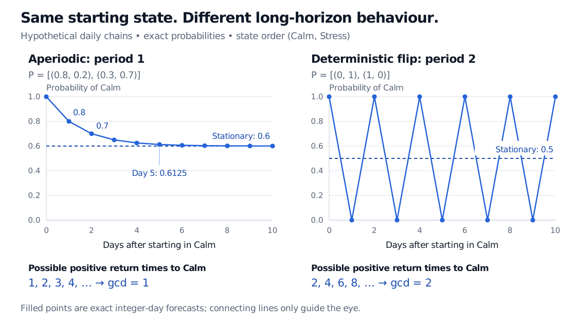
The Calm probability is therefore 0.8 after one day, 0.7 after two and 0.6125 after five, approaching 0.6. A risk calculation that combines regime-specific losses should use the relevant finite-horizon weights; replacing them immediately with 60% Calm and 40% Stress discards information about today's state. Aperiodicity permits convergence here, but the rate comes from this particular matrix.
Exact Calm forecast probabilities at integer days. The aperiodic daily model starts at 1, reaches 0.8 at day 1, 0.7 at day 2 and 0.6125 at day 5, approaching 0.6. A deterministic flip alternates 1 and 0 forever despite stationary Calm probability 0.5.
Hypothetical daily chains, both starting in Calm. Filled points are exact forecast probabilities at integer days; connecting lines guide the eye. The lower labels identify the complete sets of possible positive return times to Calm.
A stationary law can coexist with oscillation
Replace the matrix by a rule that switches state with certainty:
F=(0110).
This chain is still finite and irreducible. Its unique stationary distribution is (1/2,1/2): starting with those random weights preserves them at every date. Starting definitely in Calm instead gives Calm probability one on even days and zero on odd days. Its return times are exactly 2,4,6,…, so the period is two and this forecast never converges.
The time fraction spent in Calm nevertheless tends to one half along the alternating path. Convergence of a marginal distribution and convergence of a time average are different claims. Aperiodicity is required for the former general guarantee, not for the finite irreducible chain's long-run occupation fractions.
The assumptions can now be kept distinct:
Every finite time-homogeneous chain has at least one stationary probability distribution.
Finite and irreducible guarantees a unique stationary distribution and positive recurrence: mean return times are finite.
Adding aperiodicity guarantees that the distribution converges to that stationary law from every initial distribution.
Aperiodicity alone does not give a unique long-run law. The two-state identity matrix has self-loops of probability one, hence period one at both states, but every initial distribution is stationary. In a countably infinite irreducible chain, finiteness no longer supplies positive recurrence: a stationary probability law requires that extra condition. With positive recurrence and aperiodicity, convergence follows. MIT's countable-state notes state this version explicitly.
Richard Durrett, Essentials of Stochastic Processes, third edition (Springer, 2016), §1.6, especially Lemmas 1.17–1.18 and Theorems 1.19–1.22: periods, self-loops, convergence and occupation frequencies.
John Sylvester, Nicolás Rivera, Luca Zanetti and Thomas Sauerwald, Lecture 2: Markov Chains, University of Cambridge, Lent 2019, slides 13–18: stationary distributions, periodicity and finite-state convergence.