A stopping time can be recognised using information available so far. Test a capped profit-taking rule, a hindsight-based last visit and the limits of optional stopping.
Stopping time
A stopping time is a random time whose occurrence can be recognised from the information available by then. At every time t, you must be able to answer “Have I stopped yet?” using what you currently know. You need not know in advance when stopping will happen.
This is the information constraint behind an executable exit rule or an American option exercise policy. “Sell at the first observed price above my threshold” passes the test. “Sell at the highest price this week” generally requires hindsight.
The event to test
Let (Ft) be a filtration, describing information as it arrives. A nonnegative random time τ, allowed to equal ∞, is a stopping time relative to that filtration if
{τ≤t}∈Ftfor every t.
The event inside the braces means “stopping has occurred by t.” In discrete time, checking {τ=n}∈Fn at each integer n is equivalent. A fixed deadline is also a stopping time: randomness is allowed, rather than required. The value ∞ means the rule never triggers.
The filtration is part of the claim. A rule may fail with only observed prices but pass if future prices are revealed at the start. That enlarged information would not justify implementing it in an ordinary backtest; it would encode look-ahead bias.
Take a profit, with a deadline
Consider an exact synthetic model with a price starting at USD 100. At each of two steps it independently rises or falls by USD 1, each with probability 1/2. Information reveals one move per step. This finite random walk has four equally likely complete paths.
Use the rule: stop at the first observed USD 101 price, or at step 2 if it has not been reached. Formally,
H=inf{n∈{1,2}:Sn=101},τ=min(H,2),
where the infimum of an empty set is ∞. Here H=∞ means no hit within the two monitored steps; it says nothing about an extension beyond the model's horizon. This is a capped hitting time.
Complete path
Observed prices (USD)
Stop τ
Price at exit (USD)
UU
100 → 101 → 102
1
101
UD
100 → 101 → 100
1
101
DU
100 → 99 → 100
2
100
DD
100 → 99 → 98
2
98
At time 0 nobody has stopped. At time 1, {τ≤1} is exactly “the first move was U,” an observed event. At time 2 everyone has stopped. Thus the rule passes the stopping-time test at every date in this model.
The stopped process freezes the recorded value after exit:
Snτ=Smin(n,τ).
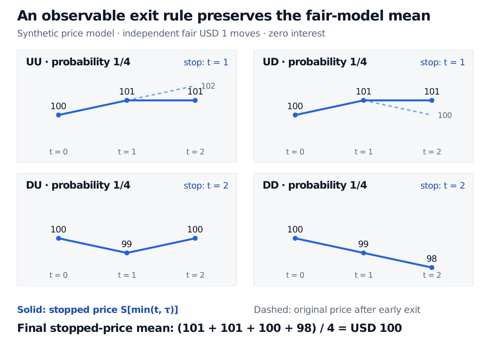
On UD, for instance, the original price ends at USD 100 while the stopped process stays at USD 101. This is a mathematical record of the stopped price. Treating it as actual liquidation wealth would additionally require an execution and cash-account model; the illustration assumes zero interest and ignores trading costs.
Four equally likely paths start at USD 100 with independent USD 1 moves. UU and UD stop at step 1 at USD 101; DU and DD stop at step 2 at USD 100 and USD 98. Their stopped-price mean is USD 100.
Original exact synthetic model, with prices in USD. Solid lines show the stopped process; dashed lines show the original price's continuation after an early stop. Each complete path has probability 1/4.
A last visit fails the same test
On the same four paths, define L as the last time the price equals USD 100 among times 0, 1 and 2. Every path has an initial visit, so L is well defined.
On UU and DD, L=0.
On UD and DU, L=2.
At time 0, the price is USD 100 on every path. Yet the event {L≤0} selects UU and DD: precisely the paths that will never revisit USD 100 within the horizon. That event cannot be decided from the common initial information. L is not a stopping time for the observed-price filtration.
Knowing at time 2 which earlier date was the last visit does not repair the failed decision at time 0. This is why labelling an exit retrospectively is a different operation from specifying a usable stopping rule.
Stopping fairly does not guarantee a profit
Under the stipulated fair-move probabilities, Sn is a martingale: the conditional expected next price equals the current price. Our rule is bounded by 2, so the bounded optional stopping theorem applies. Its expected value at exit is
E[Sτ]=21(101)+41(100)+41(98)=100.
The rule takes a USD 1 gain on half the paths, breaks even on a quarter, and loses USD 2 on a quarter. The expected change remains zero before costs. A valid stopping time supplies the information condition; martingale and horizon or integrability conditions supply the expectation result. Being a stopping time alone says nothing about whether the underlying has positive drift or whether the rule is profitable.
For an unbounded stopping time, even almost-sure eventual stopping is insufficient to assert E[Mτ]=E[M0] for a martingale M. Additional conditions controlling the stopped values are needed. Continuous-time results also require appropriate process regularity; the finite example here avoids those extra issues.
In option pricing, stopping-time admissibility similarly comes before optimisation. An exercise policy must use current information; choosing the best admissible policy then compares immediate payoff with continuation value. American Options and Early Exercise develops that comparison and its backward recursion. The public page provides a preview; the full lesson requires membership.
Sources
Gregory F. Lawler, Stochastic Calculus: An Introduction with Applications, revised February 15, 2023, §1.3, especially Theorem 1.3.1 — discrete stopping times, stopped martingales and the bounded-horizon expectation result.
Steven E. Shreve, Stochastic Calculus and Finance, CMU lecture notes by Prasad Chalasani and Somesh Jha, July 25, 1997, §5.2 — stopping-time exercise rules and the failure of hindsight-based extrema. These are the 1997 notes, rather than the later textbook.
James Norris, Advanced Probability, §2.2 — the information-event definition, stopped processes and bounded optional stopping. The four-path example and figure above are original.