Portfolio optimisation chooses asset weights for a stated objective and constraints. Work through minimum variance, a return floor, infeasible targets and sensitivity to estimated inputs.
Portfolio optimisation
Portfolio optimisation chooses the weights of a portfolio to achieve a stated objective while satisfying investment restrictions. The answer depends on what “best” means: minimum variance, a return target with the least risk, a trade-off between expected return and risk, or a different criterion such as losses relative to a benchmark.
An optimiser needs three things: decision variables such as asset weights, an objective function to rank portfolios, and constraints describing what may be held. It also needs inputs—forecasts, a risk model and any trading-cost estimates. Solving the resulting problem accurately does not make those inputs accurate.
From investment question to mathematical problem
In one-period mean–variance optimisation, let w contain the asset weights, μ their estimated expected returns and Σ their estimated covariance matrix. The two summaries are
μp=w⊤μ,σp2=w⊤Σw.
Here μp is expected return, and σp is the standard deviation of return, commonly called volatility. The formulas aggregate simple returns using weights measured at the start of the period. A weighted average of log returns is generally not the portfolio's log return.
One possible investment question is: Which fully invested, long-only portfolio has the smallest variance while offering at least a specified expected return? Its formulation is
wminsubject tow⊤Σw1⊤w=1,wi≥0for every asset i,w⊤μ≥rmin.
The first restriction spends the entire portfolio budget; the second prohibits short positions. Together they also prevent borrowing to buy more than 100% in risky assets. The last restriction is a minimum model expectation, not a floor under the money eventually earned. This is a convex quadratic programme when the covariance matrix is positive semidefinite and the restrictions are linear. The moment formulas require finite second moments, but do not require normally distributed returns. The CVX Short Course develops these formulations.
Two assets, two different answers
Suppose a small investment committee is comparing two fictional funds. It uses these illustrative inputs, all over the same one-year horizon, in a common currency:
Input
Fund A
Fund B
Expected simple total return
8%
4%
Return volatility
20%
10%
Their covariance is assumed to be zero. These are stipulated model estimates, not observed market quotes. Weights are continuous fractions of initial wealth, held for the year without rebalancing. There is no cash asset, shorting, borrowing, transaction cost, management fee or tax; returns include distributions and are gross of those costs.
Write w for A's weight and 1−w for B's. Long-only, fully invested portfolios have 0≤w≤1. Using decimal returns,
μp(w)=0.04+0.04w,v(w)=0.04w2+0.01(1−w)2.
The variance coefficients are squared volatilities: 0.202=0.04 and 0.102=0.01. The cross term disappears because covariance is zero; zero covariance alone does not imply independence.
First ask only for minimum variance. Completing the square gives a global certificate:
v(w)=0.008+0.05(w−0.20)2.
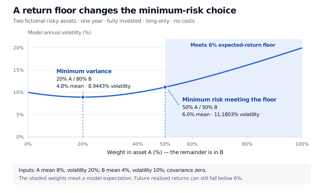
Every departure from w=0.20 adds a nonnegative amount to variance. The minimum is therefore 20% A and 80% B, with expected return 4.8%, variance 0.008 and volatility 8.9443%. Even though A is more volatile, holding some A reduces portfolio variance below B's variance through diversification.
Now require at least 6% expected return. The new constraint is
0.04+0.04w≥0.06⟺w≥0.50.
The 20/80 mix is no longer feasible. Variance increases as w moves above 0.20, so the least-risk permitted choice is 50% A and 50% B. It has expected return 6%, variance 0.0125 and volatility 11.1803%. The higher return requirement has bought a different model trade-off, with more volatility.
Synthetic annual volatility versus weight in A: minimum volatility 8.9443% at 20% A, while a 6% expected-return floor requires at least 50% A and raises minimum volatility to 11.1803%.
Original synthetic one-year simple-return model. Fully invested long-only inception weights; no cash, rebalancing or costs. The shaded region meets an expected-return constraint, which does not guarantee a realised return.
A minimum-return restriction need not bind. If the committee instead asked for at least 4.5%, the 20/80 portfolio would remain optimal and would still offer a model mean of 4.8%. Forcing the mean to equal 4.5% would solve a different problem.
Feasible alternatives are part of the answer
The feasible set contains every portfolio meeting all restrictions. Under the 6% floor, it contains every A weight from 50% through 100%. These alternatives all qualify; they do not all minimise variance.
Portfolio
Model expected return
Model volatility
Meets 6% floor?
20% A / 80% B
4.8%
8.9443%
No
50% A / 50% B
6.0%
11.1803%
Yes; minimum variance among qualifying weights
100% A
8.0%
20.0000%
Yes
Maximising expected return alone would select 100% A under the original budget and long-only rules. Choosing 50/50 instead reflects a risk objective. Varying the return requirement traces the relevant part of the efficient frontier, rather than revealing one universally best portfolio.
Restrictions can also make the request impossible. A cap of 40% in A limits the expected return to 5.6%. With that cap, a 6% floor has no feasible solution. The correct response is to revisit the target, universe or permitted holdings. An algorithm cannot satisfy inconsistent instructions by searching harder.
The inputs deserve as much scrutiny as the solver
Revise only A's expected return from 8% to 7%, leaving the volatilities and zero covariance unchanged. The existing 50/50 portfolio now has an expected return of 5.5%. Meeting the same 6% floor requires two-thirds in A, with one-third in B. The optimiser increases exposure to the asset whose forecast was lowered because the committee has kept its target fixed. That is a consequence of the chosen problem.
In practice, historical samples, forecasting models and covariance estimates can disagree or change. Optimisation can concentrate on apparently attractive estimates that contain substantial error. Ledoit and Wolf explain this estimation-error problem and motivate covariance shrinkage. Shrinkage, position limits and scenario comparisons can help control sensitivity; none turns an estimated mean into a promised return.
Trading adds another decision: whether moving from the current holdings to the proposed weights is worth the cost. A repeated cost-free optimisation may propose frequent changes whose forecast benefit disappears after spreads, fees and market impact. A trading formulation needs current holdings, a cost model and a budget that pays those costs; Boyd and co-authors describe how return, risk, trading costs and holding costs enter that problem.
A useful result therefore reports the objective, horizon and return convention; the inputs and their estimation method; the weights and constraint residuals; and sensitivity to plausible input changes. A numerically optimal weight vector is a conditional answer to that specification. Variance also treats favourable and unfavourable deviations alike, so a variance minimum alone does not establish protection against drawdowns, illiquidity or extreme losses.
For the matrix derivations and benchmark-relative extension, continue with Mean-Variance Optimisation (membership for the full lesson; public preview).
Sources
Edward E. Qian, Ronald H. Hua and Eric H. Sorensen, Quantitative Equity Portfolio Management: Modern Techniques and Applications, Chapman & Hall/CRC, 2007, Chapter 2 introduction and §§2.1–2.2: portfolio moments, minimum variance and expected-return forecasts.