Fit one polynomial through distinct data points, see an exact positive-knot example turn negative, and understand the role of degree, node placement and curve constraints.
Polynomial interpolation
Polynomial interpolation finds a polynomial that passes exactly through supplied data points. With n+1 distinct input nodes, there is exactly one such polynomial of degree at most n.
A quant can use this to fill a valuation grid between expensive model runs. But exact agreement at the grid points does not ensure sensible values between them: even positive supplied responses can produce a negative interpolated value.
What the degree limit buys
For nodes x0,…,xn and responses y0,…,yn, the conditions are
pn(xi)=yi,i=0,…,n.
The degree can be lower than n; constant or collinear data do not require a high-degree curve. Uniqueness follows because the difference of two candidates would have n+1 distinct roots while having degree at most n.
Without the degree restriction, the data do not identify a unique polynomial. For any nonzero constant c,
q(x)=pn(x)+ci=0∏n(x−xi)
still passes through every node. Repeated input locations also need care: different responses at the same input are inconsistent with a single function, while repeating the same pair adds no constraint.
Lagrange interpolation constructs the unique degree-bounded polynomial using cardinal basis functions. Newton interpolation represents that same polynomial with divided differences. They are representations of one mathematical answer, rather than competing rules for the values between identical knots. By contrast, linear interpolation applied separately between adjacent knots generally produces a different curve.
Five positive observations, a negative answer
Consider the synthetic, dimensionless Runge function
f(x)=1+25x21,−1≤x≤1.
It is positive throughout this interval. Sample it at five equally spaced nodes:
Input xi
Response yi=f(xi)
−1
1/26
−1/2
4/29
0
1
1/2
4/29
1
1/26
Symmetry lets us seek an even quartic, p4(x)=1+ax2+bx4. Imposing the values at 1/2 and 1 gives
p4(x)=1−7543225x2+3771250x4.
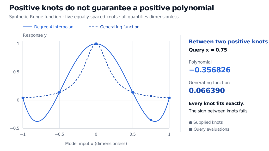
This fits all five observations exactly. Yet at x=3/4, inside the last pair of knots,
The sign failure exists in exact arithmetic. More digits or a different representation of this same polynomial cannot remove it. This is an interpolation-choice problem, even when the evaluation algorithm is accurate.
Five positive Runge-function knots at minus 1, minus 0.5, 0, 0.5 and 1 are fitted exactly by one quartic. At x=0.75 the quartic gives minus 0.356826 while the generating function gives 0.066390.
Original synthetic example, with dimensionless inputs and responses. Filled circles are supplied knots; filled squares mark the two query evaluations. The solid quartic crosses below zero despite fitting every positive knot; the dashed generating function stays positive.
The known function supplies a benchmark here. With only observed knots, its between-knot values would be unknown: choosing an interpolant does not create additional observations. If the response represented a quantity required to be nonnegative, this quartic would fail that requirement. The example is not a model of market prices.
Accuracy depends on the function and the nodes
If the data are exact samples of a function with a continuous (n+1)st derivative on an interval containing the nodes and query, then at a non-node query
f(x)−pn(x)=(n+1)!f(n+1)(ξ)i=0∏n(x−xi)
for some ξ in that interval. Both the derivative and the node product matter. Merely increasing the number of equispaced knots does not establish that this error decreases.
The Runge phenomenon describes how increasing the degree with equispaced nodes can produce worsening oscillations, particularly near interval ends. The single quartic above illustrates overshoot; one finite-degree example alone does not demonstrate the limiting behaviour as the degree grows. When sampling locations are controllable, Chebyshev interpolation uses endpoint-clustered nodes to improve the geometry. It does not make arbitrary fixed market maturities movable.
Choose a construction and a financial contract
For evaluating a global polynomial, barycentric interpolation avoids explicitly expanding it into monomial coefficients. A careful implementation returns the supplied value at an exact node. Such computational choices help control arithmetic error; they cannot fix the negative value of the exact quartic above or eliminate poor conditioning.
For a large supplied grid, a cubic spline keeps the degree low on each interval. If preserving local direction and range is essential, monotone interpolation addresses a different requirement from smooth knot fitting. Neither a generic spline nor a polynomial fit automatically certifies financial no-arbitrage.
The quantity being interpolated matters too. SelfMadeQuant's Object-Oriented Model Design builds a discount-curve object that interpolates log discount factors, keeps discount factors positive, and rejects queries outside its maturity range. Its preview is public; the full lesson requires membership. It shows how a chosen interpolation rule becomes part of a valuation interface, rather than teaching the global polynomial construction.
Finally, evaluating a fitted curve beyond its outer nodes is extrapolation. Exact knot matching supplies no general guarantee there either.