Newton interpolation: Definition & Examples

Newton interpolation expresses the polynomial through a set of data points as a sum of successively higher-degree terms, with coefficients given by divided differences. It is useful when a valuation needs a function value between supplied knots: for example, a rate at a maturity where no knot was supplied.

With

n+1

distinct nodes, the polynomial interpolant has degree at most

n

. Newton's form makes it easy to append a node while retaining the existing coefficients. It constructs a curve; Newton–Raphson instead iterates towards a root of an equation. The shared name does not make them the same algorithm.

A rate between three knots

Consider this synthetic set of continuously compounded annual zero rates. Maturity is measured in years; no calendar day-count adjustment is involved.

Maturity	Rate	Role
0 years	2%	Supplied hypothetical short-end anchor
1 year	2.5%	Supplied knot
2 years	3.5%	Supplied knot

The 0-year entry is a stipulated limiting-rate anchor. A bond paying immediately has discount factor one regardless of the rate; its price cannot reveal a 0-year yield.

Write

R(t)

for the numerical rate in percent units, so

R(1)=2.5

means 2.5%, not 250%. The first divided differences are the changes in the rate divided by changes in maturity:

R[0,1]=\frac{2.5-2}{1-0}=0.5, \qquad R[1,2]=\frac{3.5-2.5}{2-1}=1.

The second divided difference compares these slopes over the full node span:

R[0,1,2]=\frac{R[1,2]-R[0,1]}{2-0} =\frac{1-0.5}{2}=0.25.

The Newton polynomial is therefore

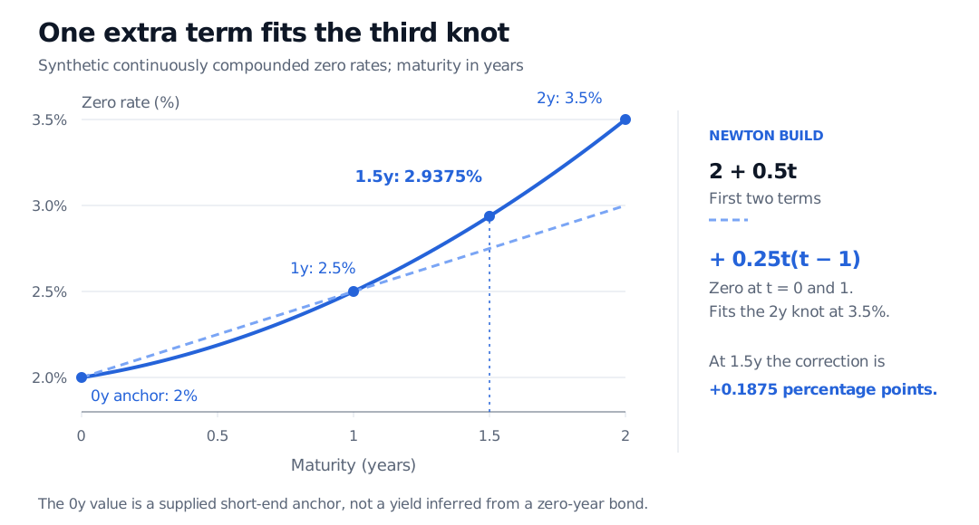
P_2(t)=2+0.5t+0.25t(t-1).

The first term fixes the anchor. The next term fits the 1-year knot. The last term vanishes at both earlier nodes, so it can fit the 2-year knot without disturbing them. Substitution gives $P_2(0)=2$ , $P_2(1)=2.5$ and $P_2(2)=3.5$ .

At 1.5 years,

P_2(1.5)=2+0.75+0.1875=2.9375.

Thus the interpolated zero rate is 2.9375%, or 0.029375 in decimal form. The correction of 0.1875 is in percentage points. It is added to the first two terms' value of 2.75%, not multiplied by that rate.

The Newton quadratic passes through synthetic rate knots 2%, 2.5% and 3.5% at 0, 1 and 2 years. At 1.5 years it gives 2.9375%, versus 2.75% for the first two terms. The zero-year value is a supplied anchor.

Original synthetic curve. The solid line includes the quadratic correction; the dashed line shows only the first two Newton terms. Filled markers show attained values. The 0-year rate is supplied, not inferred from a bond price.

Units travel with the coefficients. With maturities in years and rates in percent units, the coefficients have units of percentage points, percentage points per maturity-year, and percentage points per maturity-year squared, respectively. Using decimal rates divides all three coefficients by 100:

p_2(t)=0.02+0.005t+0.0025t(t-1).

For positive maturity, the corresponding continuously compounded discount factor would be $D(t)=\exp[-t\,p_2(t)]$ . Putting $P_2(t)$ directly into that exponent would mix percent and decimal conventions.

Why the representation is convenient

For data $(x_i,y_i)$ , write $f[x_i]=y_i$ and recursively define

f[x_i,\ldots,x_{i+k}] =\frac{f[x_{i+1},\ldots,x_{i+k}]-f[x_i,\ldots,x_{i+k-1}]}{x_{i+k}-x_i}.

The coefficients $a_k=f[x_0,\ldots,x_k]$ give

P_n(x)=a_0+\sum_{k=1}^{n}a_k\prod_{j=0}^{k-1}(x-x_j).

Each new product is zero at all preceding nodes. Appending one node therefore needs one additional term, with the earlier coefficients unchanged. Nodes need not be equally spaced. They must be distinct for this recurrence; repeated-node interpolation requires additional information, such as derivatives in Hermite interpolation, and a different treatment.

Changing node order changes the Newton basis and generally its coefficient sequence. Reversing this example's order to 2, 1, 0 gives

P_2(t)=3.5+(t-2)+0.25(t-2)(t-1).

It is still

2+0.25t+0.25t^2

. The exact polynomial also equals the Lagrange interpolant for the same points: uniqueness fixes the curve, while the representation determines how it is computed. Rounding error can make finite-precision results depend on order.

An exact fit is only one requirement

The example interpolates zero rates. Interpolating discount factors, their logarithms or forward rates would generally produce different values between the same maturities. That choice affects valuations and sensitivities. SelfMadeQuant's Object-Oriented Model Design lesson implements a curve with log-linear discount-factor interpolation and an explicit rule for out-of-range requests. Its preview is public; the full lesson requires membership.

A global polynomial can oscillate as its degree grows; exact agreement at the knots does not control behaviour between them. Extrapolation beyond the outer nodes adds further risk. Newton's basis does not automatically cure poor conditioning or guarantee a stable computation.

Nor does an arbitrary interpolated rate polynomial establish an arbitrage-free yield curve. A usable curve needs coherent conventions, checks on implied discount and forward rates, and consistency with the instruments it is intended to price. The interpolation calculation alone provides none of those financial guarantees.

Sources

NIST Digital Library of Mathematical Functions, §3.3(iii)–(iv), divided differences and Newton's interpolation formula.
Tobin A. Driscoll and Richard J. Braun, Fundamentals of Numerical Computation, §9.1, uniqueness and the Lagrange representation.
Rüdiger U. Seydel, Tools for Computational Finance, sixth edition, Springer, 2017, Appendix C.1, “Interpolation”, pp. 420–421: polynomial and piecewise interpolation in computational finance.

A rate between three knots

Why the representation is convenient

An exact fit is only one requirement

Sources

Related terms

Newton-Raphson method

Numerical conditioning

Rounding error

Yield curve