Extrapolation estimates a function outside the range of its input data by extending a chosen rule. A desk valuing a three-year cash flow from rates supplied only through two years must decide how the curve continues. Matching every supplied point does not determine that continuation.
Interpolation fills gaps within the input range. Extrapolation crosses its boundary. The distinction concerns the input variable: extending today's curve to a longer maturity is extrapolation across maturities, not automatically a forecast of what rates will be next year.
Two quotes cannot choose a tail
Suppose a synthetic yield curve supplies annual continuously compounded zero rates of 2% at one year and 3% at two years. Let be the numerical maturity in years, with rates expressed as decimals.
Extending the straight line through these points gives
But another candidate is
The added term vanishes at both supplied maturities. Both curves reproduce the two quotes exactly, yet their three-year rates differ by two percentage points. They also differ between the knots: the example proves agreement at supplied points, not agreement throughout the observed interval. Neither curve is presented as a market forecast or an arbitrage-free curve construction.
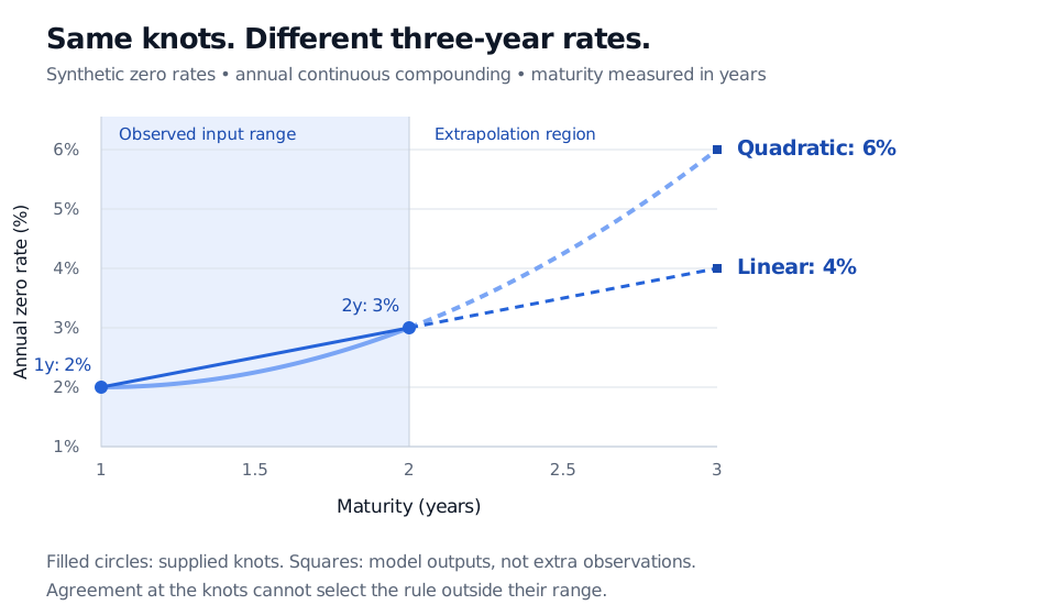
Original synthetic curves. Shading marks the input range; dashed lines mark extrapolation. Agreement at the knots cannot select the continuation.
The valuation consequence is immediate. With continuous compounding, the discount factor is . For a default-free payment of USD 100 at three years, the two stipulated rules give:
| Rule | Three-year zero rate | Present value, USD |
|---|---|---|
| Linear extension | 4% | |
| Quadratic extension | 6% |
The difference is USD 5.17, calculated before rounding the two prices. An exact fit at the input knots has left meaningful model risk in the unobserved region.
The membership lesson Bond Prices, Discount Factors, and the Law of One Price develops how maturity-specific discount factors value individual payments and coupon bonds. Its public page provides a preview; the full lesson requires membership.
Why the boundary matters
For two points and , with , the affine rule can be written
Inside the interval, both weights are nonnegative and sum to one. Outside it, one weight is negative. At with knots at one and two, the weights are and : the estimate is . A one-basis-point change in the second quote, holding the first fixed, moves this estimate by two basis points. This is sensitivity to the inputs, separate from the uncertainty about which extension rule is appropriate.
There is no universal extrapolation error bound from those two quotes alone. A bound needs additional assumptions, such as a controlled derivative over the entire interval reaching the query point. Smoothness inside the supplied range does not establish the behaviour outside it.
Specify the continuation, not just the interpolator
A usable curve specification says what is extended, by which rule, and how far. A flat zero rate, a flat forward rate and a linear discount factor impose different assumptions. A limit or economic restriction can be useful evidence for a tail, but it must be supplied separately from the finite observations.
Software behaviour deserves the same care. SciPy documents different controls for out-of-range evaluation across interpolation routines. A natural cubic spline has zero second derivative at its endpoints; continuing its terminal cubic polynomial can still produce a nonlinear extrapolation. An endpoint condition is not a complete tail policy. Check the actual routine, and reject or flag a query when the intended policy is absent.
Finally, Richardson extrapolation uses a different setting: it combines numerical approximations at finite step sizes to estimate a limiting value at zero step size. Its justification comes from an assumed error expansion. It does not justify extending an observed market trend indefinitely.
Sources
- Damir Filipović, Term-Structure Models: A Graduate Course, Springer, 2009, §2.2 for rate and discount-factor relationships; §3.3.1, pp. 39–42, for spline fitting and instability at the ends of the maturity range.
- SciPy: Extrapolation tips and tricks, for explicit out-of-range policies and why natural spline boundary conditions do not imply linear extrapolation.
- SciPy:
CubicSpline, for the separate boundary-condition and extrapolation controls and evaluation using the first or last polynomial interval.