Estimate values between supplied points, and see why matching every knot does not determine a unique curve or a financially valid interpolation rule.
Interpolation
Interpolation constructs values between supplied data points by choosing a function that passes through them. A quant uses it when a cash-flow date, option strike or numerical-grid query falls between available inputs. The missing value comes from an explicit modelling rule; it is not another observed quote.
For ordered nodes x0<⋯<xn with values yi, an interpolant I satisfies
I(xi)=yi,i=0,…,n.
This condition alone leaves infinitely many possible curves. Choosing straight segments, a global polynomial or a spline supplies the extra structure. Evaluating beyond the outer nodes is extrapolation, where the data no longer bracket the query.
A missing maturity is a choice
Suppose a synthetic curve supplies these annual continuously compounded zero rates. Maturities are measured in years; these are illustrative inputs, not market observations.
Maturity
Zero rate
1 year
2.00%
2 years
2.50%
3 years
3.50%
What rate should apply at 1.5 years?
Linear interpolation uses the two surrounding points. Halfway between 1 and 2 years gives
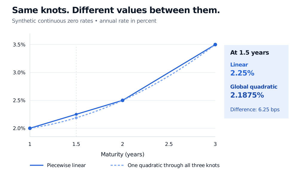
rL(1.5)=2.00%+2−11.5−1(2.50%−2.00%)=2.25%.
A different valid choice is the unique polynomial interpolant of degree at most two through all three points. Write its rate in percent units, so 2 means 2%:
q(t)=2+0.5(t−1)+0.25(t−1)(t−2).
It gives q(1.5)=2.1875, meaning a rate of 2.1875%. Both methods reproduce every supplied rate. They differ at the missing maturity by 6.25 basis points. Neither is a rounding error: they encode different assumptions about the curve between inputs.
Synthetic zero rates at 1, 2 and 3 years are 2%, 2.5% and 3.5%. The piecewise linear curve gives 2.25% at 1.5 years; the global quadratic gives 2.1875%, a difference of 6.25 basis points.
Original synthetic example. Filled knots are supplied rates; both interpolants pass through them. The curves are shown only over the supplied maturity range.
Specify the quantity before the method
“Interpolate the curve linearly” is incomplete. You could interpolate zero rates, discount factors, their logarithms or forward rates. These choices generally produce different answers because transforming a value and interpolating it do not commute.
For the first two knots above, let D(t)=e−r(t)t, with the rate now written as a decimal. Linear zero-rate interpolation gives
DL(1.5)=e−0.0225×1.5=e−0.03375.
Instead, taking the geometric midpoint of the two discount factors gives
D(1)D(2)=e−0.02e−0.05=e−0.035.
That corresponds to a 1.5-year zero rate of 0.035/1.5=2.3333% annually, rounded to four decimal places in percent units. Geometric discount-factor interpolation is linear interpolation of log discount factors, not generally of zero rates with the same weights. The maturity multiplier matters.
What should the curve preserve?
Straight segments keep the response between its two surrounding values, but their derivative can jump at a knot. A cubic spline joins polynomial pieces with continuous first and second derivatives. That extra smoothness can help when a calculation uses curve derivatives, but it requires boundary assumptions and can introduce overshoot.
The financial constraints belong to the interpolated object. For option prices across strikes, monotonicity and convexity matter; for rates, the consequences depend on the resulting discount and forward curves. Exact matching at the knots, a smooth picture and absence of arbitrage are separate requirements.
For an options application, The Black-Scholes PDE, Formula and Implied Volatility discusses filling a volatility surface between quoted strikes and maturities (membership; public preview). Treat its interpolation choices as construction choices that also need financial checks.
Finally, interpolation is not smoothing. When observations contain noise, a regression or smoothing spline may deliberately leave residuals rather than pass through every point. Zero error at the inputs establishes a fit to those inputs; it does not establish accuracy between them.
Damir Filipović, Term-Structure Models: A Graduate Course (Springer, 2009), Chapter 3 introduction and §3.1, pp. 29–33 — finite quoted maturities, off-grid cash flows and curve construction. The distinction between interpolating zero rates and log discount factors above follows directly from logD(t)=−r(t)t.