Linear interpolation: Definition & Examples

Linear interpolation estimates a value between two known points by drawing the straight line through them. With a sequence of ordered points, it joins each neighbouring pair separately: a piecewise linear curve.

For a quant, the choice is often practical rather than abstract. A discount curve may have inputs at one and three years while a cash flow arrives at two years. Linear interpolation supplies an intermediate value with a transparent calculation. It also makes an assumption: the chosen quantity changes at a constant rate within that interval. The missing quote has not become an observation.

Distance determines the weights

For $x_0<x_1$ and a query $x\in[x_0,x_1]$ , define

w=\frac{x-x_0}{x_1-x_0},\qquad L(x)=(1-w)y_0+wy_1.

The weight $w$ measures the fraction of the horizontal distance travelled from the left endpoint. It is not usually $1/2$ : only the midpoint receives equal weights. At either endpoint the formula returns the supplied value exactly.

Because

0\le w\le1

, the interpolated value lies between the two endpoint values. Positive inputs stay positive within the interval, and a monotone sequence of inputs produces a monotone piecewise linear curve. These are properties of the quantity being interpolated, not general economic guarantees for everything derived from it. Driscoll and Braun's treatment develops the piecewise construction and its stability.

Two rates, one missing maturity

Take synthetic annual continuously compounded zero rates, with maturity measured in years:

Maturity	Zero rate
$1$ year	$2\%$
$3$ years	$4\%$

At two years, $w=(2-1)/(3-1)=1/2$ , so

r(2)=\tfrac12(2\%)+\tfrac12(4\%)=3\%.

1.5

years,

w=1/4

, giving

r(1.5)=2.5\%

. The segment's slope is one percentage point per year of maturity. The rate is quoted per annum with continuous compounding; the slope describes how that quote changes as maturity changes.

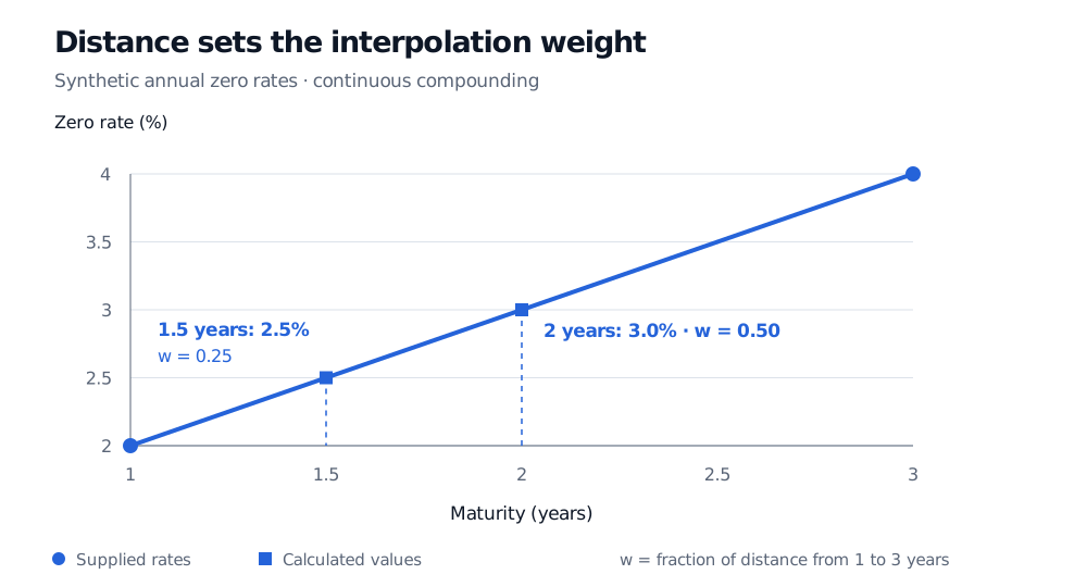
A straight rate segment joins the supplied rates 2% at one year and 4% at three years. Calculated values are 2.5% at 1.5 years with weight 0.25, and 3% at two years with weight 0.5.

Original synthetic example. Filled circles are supplied rates; filled squares are calculated values. The horizontal distance, not the number of data points, sets the weight.

Name the quantity before drawing the line

A discount factor associated with a continuously compounded zero rate is

D(t)=e^{-t r(t)}

, using decimal rates. Interpolating rates and then converting to discount factors generally differs from interpolating discount factors directly. Even interpolating their logarithms gives a third construction.

The same one- and three-year inputs imply $D(1)=e^{-0.02}$ and $D(3)=e^{-0.12}$ . At two years:

Quantity interpolated linearly	Resulting two-year discount factor
Zero rate $r$	$e^{-2(0.03)}\approx0.94176453$
Discount factor $D$	$(e^{-0.02}+e^{-0.12})/2\approx0.93355956$
Log discount factor $\log D$	$e^{(-0.02-0.12)/2}\approx0.93239382$

All three constructions match the endpoint discount factors. Their intermediate prices differ because the transformation includes both an exponential and the maturity multiplier. A specification such as “linear curve” is therefore incomplete: say linear in what. Building a yield curve also requires consistent instruments, conventions and economic constraints.

For a concrete implementation of the third choice, Object-Oriented Model Design builds a curve that interpolates log discount factors and rejects maturities outside its input range (membership; public preview).

Local simplicity has a price

With several knots, each query uses its own bracketing pair. Changing one input affects only the adjacent segments. The curve is continuous, but its derivative generally jumps where two unequal segment slopes meet. It is

C^0

, and generally not

C^1

. If a downstream calculation needs smooth derivatives, consider a cubic spline and check its boundary and shape assumptions.

Neither exact passage through the inputs nor a lack of overshoot establishes that an interpolant is accurate between sparse quotes. Unlike linear regression, interpolation does not average away observation noise or fit a trend with residuals.

Finally, a query outside the endpoint range is extrapolation. Extending the last segment, holding the last value constant and rejecting the query are different policies. For example, numpy.interp holds endpoint values by default outside the range. Validate strictly increasing finite input coordinates and choose the outside-range policy explicitly.

Sources

Cornuéjols, Peña and Tütüncü, Optimization Methods in Finance, 2nd edition (Cambridge University Press, 2018), §3.4, “Yield Curve and Term Structure,” pp. 42–43 — spot-rate construction and interpolation between observed maturities.
Driscoll and Braun, Fundamentals of Numerical Computation, §5.2: Piecewise linear interpolation — neighbouring-interval construction, continuity and conditioning.
NumPy documentation: numpy.interp — coordinate ordering and outside-range defaults.

Distance determines the weights

Two rates, one missing maturity

Name the quantity before drawing the line

Local simplicity has a price

Sources

Related terms

Cubic spline

Derivative (calculus)

Discount factor

Extrapolation

Linear regression

Yield curve