Join cubic pieces with continuous slope and curvature, and see how endpoint conditions change an exact interpolation without guaranteeing financial validity.
Cubic spline
A cubic spline is a function built from polynomial pieces of degree at most three, joined so that the value, first derivative and second derivative agree at each ordinary interior knot. The resulting curve is twice continuously differentiable, written C2.
In quantitative finance, that extra smoothness matters when a calculation differentiates a fitted curve. Connecting quoted values by straight lines produces corners; differentiating a cubic spline gives a continuous slope. That is useful structure for a yield curve or volatility smile, but it does not establish that the fitted curve satisfies financial constraints.
Matching values and matching derivatives
For interpolation, start with distinct ordered knots x0<⋯<xn and observed values y0,…,yn. On interval [xi,xi+1], write a local cubic
Si(x)=ai+bi(x−xi)+ci(x−xi)2+di(x−xi)3.
The interpolating spline must pass through both ends of each interval. At every interior knot, the left and right slopes must also match, as must the left and right curvatures. These conditions leave two degrees of freedom: there are 4n coefficients, 2n endpoint-value equations and 2(n−1) derivative-matching equations. Two suitable boundary conditions complete the construction.
“Cubic spline” therefore does not specify a unique interpolation rule on its own. Common choices include:
Boundary choice
What it specifies
Natural
The second derivative is zero at both outer knots.
The first derivative is prescribed at both outer knots. The slopes need not be zero.
Not-a-knot
The first two pieces share one cubic, and the last two pieces share one cubic, when there are enough knots.
These are conditions on the curve, not additional observations. Software defaults matter: SciPy's CubicSpline defaults to not-a-knot, rather than natural boundaries.
A three-point arch
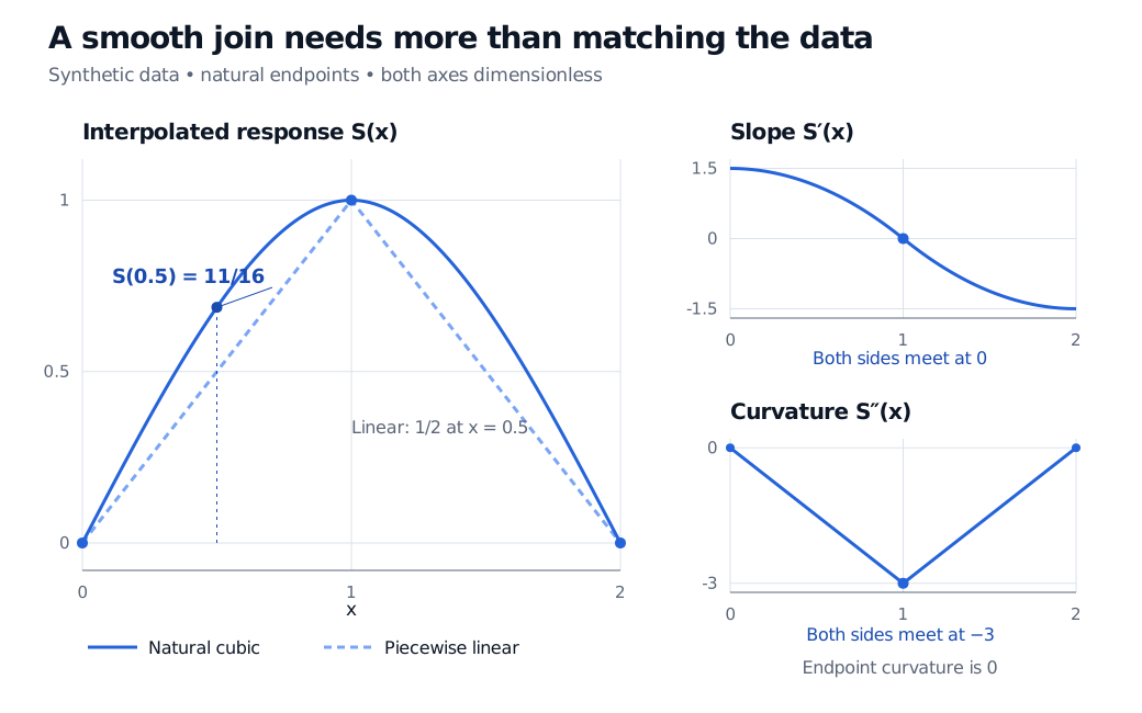
Take the synthetic, dimensionless data (0,0), (1,1) and (2,0). Impose natural boundaries S′′(0)=S′′(2)=0. The resulting spline is
S(x)={23x−2x3,23(2−x)−2(2−x)3,0≤x≤1,1≤x≤2.
At the middle knot, both expressions give value 1, slope 0 and second derivative −3. The join has no corner and no jump in curvature. The third derivative, however, jumps from −3 on the left to +3 on the right: a cubic spline need not be C3.
At x=0.5, the spline gives 11/16=0.6875, while linear interpolation gives 1/2. Both curves pass through every supplied point. Their different answers between points come from their different construction rules, not from an error in matching the data.
Synthetic natural cubic through (0,0), (1,1), (2,0), with value 11/16 at x=0.5 versus the linear value 1/2. Slope joins at zero and curvature at minus 3 at x=1; endpoint curvature is zero.
Original dimensionless example. The solid curve is the natural cubic; the dashed line connects the same data linearly. Filled markers denote attained values. The derivative panels show the two smoothness conditions at the middle knot.
Natural does not mean flat. Here S′(0)=1.5 and S′(2)=−1.5, despite zero endpoint curvature. Nor does zero curvature at the endpoint make the entire outer cubic segment a straight line.
What smoothness buys—and what still needs checking
A spline is a function class, not necessarily an exact fit. A regression spline estimates coefficients from noisy data, and a smoothing spline trades fit against a roughness penalty. Neither must pass through every observation. A B-spline is a basis for representing spline functions, rather than a competing requirement that every observation be interpolated. This distinction is developed in Hastie, Tibshirani and Friedman, Chapter 5.
Smoothness alone does not preserve monotonicity, positivity or convexity between knots. A cubic spline can overshoot; SciPy's interpolation guide illustrates this limitation. When interpolating financial quantities, specify whether the ordinate is a zero rate, discount factor, implied volatility or option price, then check the relevant pricing constraints. Changing that quantity changes the curve being constructed.
Finally, evaluating beyond the outer knots is extrapolation. Endpoint boundary conditions and the rule for extending the curve are separate choices. A smooth fit inside the observed range provides no automatic justification for its tail.
Sources
Hastie, T., Tibshirani, R. and Friedman, J. The Elements of Statistical Learning, second edition, corrected 12th printing (2017), Chapter 5, §§5.2–5.2.1 and §5.4: spline spaces, natural boundaries and smoothing splines.