Clamped cubic spline: Definition & Examples

A clamped cubic spline is a piecewise cubic interpolating curve whose first and second derivatives join continuously at the interior knots, with a prescribed first derivative at each endpoint. It passes through the supplied values and leaves the two ends with slopes you choose.

That last piece of information matters when a quant interpolates a price or term structure and then differentiates it. Two curves can match every input quote and still imply different sensitivities between quotes. Clamping makes the endpoint slope assumptions explicit; their economic justification remains a separate modelling decision.

What gets clamped?

Given distinct ordered knots $x_0<\cdots<x_n$ and values $y_i$ , the spline $S$ satisfies

S(x_i)=y_i,\qquad S'(x_0)=m_0,\qquad S'(x_n)=m_n.

Each interval has a polynomial of degree at most three. At each interior knot, the neighbouring pieces agree in value, slope and second derivative: $S\in C^2$ . The third derivative may jump. The two endpoint slopes, together with interpolation and those joins, determine a unique spline.

Here clamped does not mean flat. The numbers

m_0,m_n

may be nonzero. Nor does it mean that slopes are specified at every knot; that would be a different interpolation problem. A natural cubic spline instead sets the endpoint second derivatives to zero.

The distinction from a regression spline is equally useful. This curve interpolates its knot values exactly. In spline regression, a smooth basis is fitted to observations and generally leaves residuals. For that broader statistical use, Beyond Linearity: Splines, Local Regression, and Generalized Additive Models develops piecewise bases and model flexibility (membership; public preview).

Three values, plus two slopes

Use a synthetic, dimensionless example:

Knot $x$	Supplied value $y$
$0$	$0$
$1$	$1$
$2$	$8$

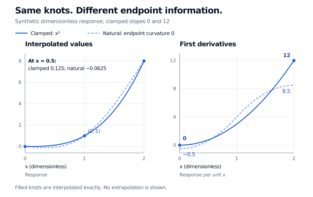
Prescribe $m_0=0$ and $m_n=12$ . The function $S(x)=x^3$ satisfies every condition: it hits the three values, its derivatives join at $x=1$ , and $S'(x)=3x^2$ gives the two required slopes. Uniqueness therefore identifies the interpolant without an approximation:

S(0.5)=\frac18=0.125, \qquad S(1.5)=\frac{27}{8}=3.375.

These three knot values alone do not identify

x^3

. Change the endpoint conditions and the interpolating curve changes. For the same data, the natural spline has

N(x)= \begin{cases} \frac32x^3-\frac12x,&0\le x\le1,\\ 1+4u+\frac92u^2-\frac32u^3,\quad u=x-1,&1\le x\le2. \end{cases}

It gives $N(0.5)=-1/16=-0.0625$ and $N(1.5)=63/16=3.9375$ . Its endpoint slopes are $-0.5$ and $8.5$ , rather than $0$ and $12$ . Neither construction has missed an input value. They solve different boundary problems.

Two panels compare clamped x cubed and the natural spline through (0,0), (1,1), and (2,8). At x=0.5 values are 0.125 and minus 0.0625. Their endpoint slopes are 0 and 12 versus minus 0.5 and 8.5.

Original synthetic example. Both curves interpolate the filled knots; the derivative panel exposes the endpoint assumptions. Coordinates and responses are dimensionless.

How the slopes enter the solve

One implementation solves for the knot second derivatives $M_i=S''(x_i)$ . Write $h_i=x_{i+1}-x_i$ and $\Delta_i=(y_{i+1}-y_i)/h_i$ . Matching first derivatives at interior knots supplies

h_{i-1}M_{i-1}+2(h_{i-1}+h_i)M_i+h_iM_{i+1} =6(\Delta_i-\Delta_{i-1}),\quad 1\le i<n.

The clamped endpoint equations are

\begin{aligned} 2h_0M_0+h_0M_1&=6(\Delta_0-m_0),\\ h_{n-1}M_{n-1}+2h_{n-1}M_n&=6(m_n-\Delta_{n-1}). \end{aligned}

In the example, the interval widths are both $1$ and the secant slopes are $1$ and $7$ . Thus

\begin{bmatrix}2&1&0\\1&4&1\\0&1&2\end{bmatrix} \begin{bmatrix}M_0\M_1\M_2\end{bmatrix} = \begin{bmatrix}6\\36\\30\end{bmatrix}, \qquad (M_0,M_1,M_2)=(0,6,12).

Those are exactly the values of $6x$ , the second derivative of $x^3$ , at the knots.

Library convention matters. In SciPy, CubicSpline(..., bc_type="clamped") means zero slopes at both ends. To supply the example's slopes, use bc_type=((1, 0), (1, 12)); the 1 denotes a first derivative. Boundary conditions and extrapolation are separate settings. A clamped fit does not supply a financially justified tail beyond the endpoint knots.

Slopes carry units and assumptions

x

is maturity in years and

y

is a decimal yield,

m

is decimal yield per year of maturity, not the yield itself. Changing the horizontal unit changes the numerical slope. Likewise, clamping an interpolated discount factor is different from clamping its logarithm or a zero rate: a derivative depends on which quantity you interpolate.

Use a clamped spline when reliable endpoint derivative information is available, for example from an analytic model or an explicitly chosen boundary rule. Estimating those slopes from sparse noisy quotes introduces another source of uncertainty. Check how changing them affects the fitted curve and the quantities derived from it.

Smoothness alone does not guarantee positivity, monotonicity, convexity or absence of arbitrage. The natural comparison above even dips below zero between nonnegative values. A clamped spline also has no general shape guarantee. Choose an interpolation method and any economic constraints together, and check them throughout the relevant domain rather than only at the knots.

Practice: change the clock

A curve is parametrised by maturity

t

in years, and a prescribed endpoint slope is

6

response units per year. You switch to

q=12t

, maturity in months, without changing the curve. What slope must the new interpolator receive?

Answer. It must receive

6/12=0.5

response units per month. If

G(q)=S(q/12)

, the chain rule gives

G'(q)=S'(q/12)/12

. Keeping the input slope at

6

would impose a slope of

72

response units per year, changing the boundary condition and generally the whole interpolant.

Sources

Driscoll and Braun, Fundamentals of Numerical Computation, §5.3: Cubic splines — piecewise cubic construction, continuity constraints and the two additional endpoint conditions.
SciPy documentation: CubicSpline — derivative boundary inputs, the zero-slope clamped shortcut and independent extrapolation control.
Hastie, Tibshirani and Friedman, The Elements of Statistical Learning, 2nd edition, corrected 12th printing (2017), §§5.2–5.2.1, pp. 143–145 — cubic spline smoothness, basis representation and the distinction between regression splines and boundary restrictions.

What gets clamped?

Three values, plus two slopes

How the slopes enter the solve

Slopes carry units and assumptions

Practice: change the clock

Sources

Related terms

Derivative (calculus)

Natural cubic spline