Interpolate with zero endpoint second derivatives, and see why a natural boundary condition guarantees neither flat slopes, monotonicity nor linear extrapolation.
Natural cubic spline
A natural cubic spline is a cubic spline whose second derivative is zero at both boundary knots. In exact interpolation, it passes through every supplied value, joins neighbouring cubic pieces with continuous first and second derivatives, and satisfies
S′′(x0)=S′′(xn)=0.
This gives a smooth curve without asking the user to supply endpoint slopes. For a quant filling gaps in a yield curve or volatility smile, however, “natural” describes a boundary assumption. It does not establish that the interpolated values are positive, monotone or financially admissible.
Zero curvature is not a flat endpoint
Here “curvature” means the second derivative, S′′. Setting it to zero says that the slope has zero instantaneous rate of change at the endpoint. It leaves the slope itself free. A clamped cubic spline, by contrast, prescribes the first derivative at each endpoint.
The natural conditions apply at two points. They do not force an entire outer interval to be linear. This is the numerical boundary condition used by SciPy's CubicSpline; its default boundary condition is not-a-knot, so natural interpolation must be selected explicitly.
A smooth curve that initially goes the wrong way
Take three synthetic, dimensionless knots:
(x0,y0)=(0,0),(x1,y1)=(1,1),(x2,y2)=(2,8).
The supplied values increase. The natural interpolant is nevertheless negative just to the right of the first knot:
At the join, both pieces have value 1, slope 4 and second derivative 9. At the two outer knots, the second derivative is zero, while the slopes are
S′(0)=−21,S′(2)=217=8.5.
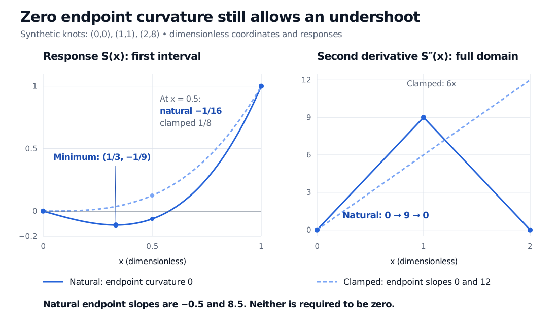
The negative initial slope makes the curve fall before it rises. Its first-interval minimum occurs at x=1/3, with value −1/9. In particular, S(0.5)=−1/16=−0.0625; further along, S(1.5)=63/16=3.9375.
For comparison, clamp the endpoint slopes to 0 and 12. The unique interpolant through the same knots is then x3, giving 1/8 at 0.5 and 27/8 at 1.5. Both curves hit all the data. Their disagreement between knots measures the effect of the boundary information.
Natural spline through (0,0), (1,1), (2,8) dips to minus 1/9 at x=1/3 and has value minus 1/16 at x=0.5, versus clamped value 1/8. Natural second derivatives at the knots are 0,9,0; endpoint slopes are minus 0.5 and 8.5.
Original synthetic example, with dimensionless coordinates and responses. The left panel magnifies the first interval; the right panel shows second derivatives over the whole domain. Filled markers denote attained values. The dashed comparison uses endpoint slopes 0 and 12.
The consequence for a financial application is concrete: nonnegative observations do not ensure a nonnegative interpolant, and increasing observations do not ensure a monotone curve. If the ordinate represents discount factors, option prices or implied volatilities, check the constraints appropriate to that quantity. Exact interpolation and smoothness alone do not provide an arbitrage-free construction.
How the boundary conditions enter the solve
One convenient construction solves for the knot second derivatives Mi=S′′(xi). Write hi=xi+1−xi. Continuity of the first derivative gives the interior equations
Natural boundaries supply M0=Mn=0, completing a tridiagonal linear system. In the example, the only interior equation is 4M1=6(7−1), hence M1=9. Integrating the linear second derivative on each interval and matching the supplied values gives the pieces above. With only two knots, zero second derivatives at both ends force the single piece to reduce to the straight line between them.
Decide what happens outside the knots
Extrapolation is a separate decision. Extending the example's final cubic to x=3 gives 15. Extending its endpoint tangent line instead gives 8+8.5(3−2)=16.5. Both extensions attach smoothly in value, slope and second derivative at x=2, but they are different curves beyond it. SciPy's extrapolation guide explains why a natural boundary condition alone does not make polynomial-piece extrapolation linear.
In statistical modelling, “natural cubic spline” often denotes a regression basis with linear tails outside the boundary knots, as in Hastie, Tibshirani and Friedman, §5.2.1. Those linear tails are an explicit extension convention. Also distinguish exact interpolation from regression: fitting a natural-spline basis to noisy observations does not generally pass through every observation.
Hastie, T., Tibshirani, R. and Friedman, J. The Elements of Statistical Learning, second edition, corrected 12th printing (2017), Chapter 5, §§5.2–5.2.1, pp.142–146: spline spaces and natural regression splines with linear tails.