Monotone interpolation: Definition & Examples

Monotone interpolation constructs a curve through ordered data points while preserving their increasing or decreasing direction between the points. If

x_0<\cdots<x_n

and

y_0\le\cdots\le y_n

, a nondecreasing interpolant

I

satisfies

I(x_i)=y_i, \qquad u<v\implies I(u)\le I(v), \quad u,v\in[x_0,x_n].

“Monotone” here allows flat stretches. The decreasing version reverses the inequality. The purpose is to stop an interpolation method introducing a turn that the supplied values do not contain.

That matters when interpolating cumulative probabilities for a risk calculation: an interpolated probability must not fall as the loss threshold rises. Passing through valid points is insufficient if the curve misbehaves between them.

The plateau test

Take three synthetic, dimensionless knots:

(0,0)

(1,1)

and

(2,1)

. The response rises, then stays level. A monotone interpolant must remain exactly 1 throughout $[1,2]$ : monotonicity traps every intermediate value between the two equal endpoint values.

Linear interpolation does this immediately, but has a corner at

x=1

. A shape-preserving PCHIP interpolant provides a continuously differentiable alternative. Using the standard shape-preserving endpoint rule, its knot slopes are

3/2

0

and

0

, giving

P(x)= \begin{cases} \frac32x-\frac12x^3,&0\le x\le1,\\ 1,&1\le x\le2. \end{cases}

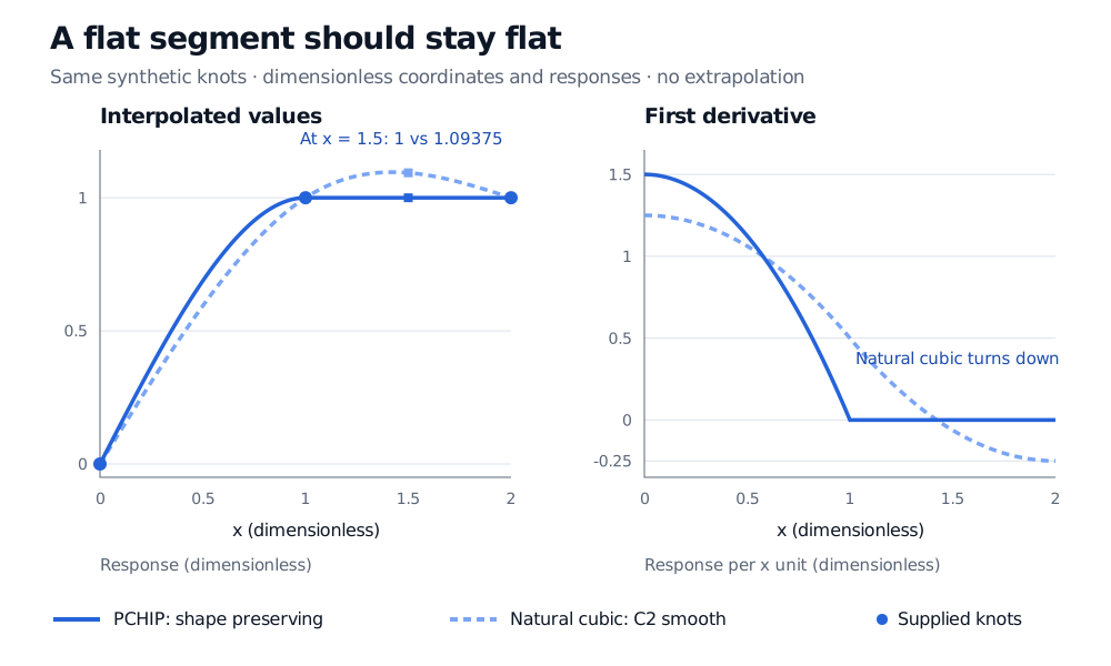
The first piece has $P'(x)=\tfrac32(1-x^2)\ge0$ on $[0,1]$ ; the second has zero slope. Both slopes meet at zero. In particular,

P(0.5)=\frac{11}{16}=0.6875, \qquad P(1.5)=1.

Now impose the boundary conditions of a natural cubic spline on the same knots. On the second interval, writing

u=x-1

, the result is

N(x)=1+\frac12u-\frac34u^2+\frac14u^3, \qquad 0\le u\le1.

At $x=1.5$ , it gives $N(1.5)=35/32=1.09375$ . Its slope there is $-1/16$ : it has risen above the plateau and is coming back down. This is an overshoot of $3/32=0.09375$ response units. If these values represented cumulative probabilities, the excursion above 1 and the subsequent decline would both be invalid.

Synthetic knots (0,0), (1,1), (2,1). PCHIP stays at 1 after x=1, while the natural cubic gives 1.09375 at x=1.5 and then decreases. A second panel compares their first derivatives.

Original synthetic comparison, with dimensionless coordinates and responses. Filled circles are supplied knots. Continuous first derivatives do not by themselves prevent a shape violation; the derivative's sign matters.

Shape is a constraint; smoothness is another

A monotonicity guarantee does not identify a unique interpolating curve. Straight segments, slope-limited cubics and other constructions can satisfy the same ordering constraint.

PCHIP chooses local cubic Hermite pieces and limits their knot slopes. An interior slope becomes zero beside a flat secant or a change of direction; otherwise a weighted harmonic mean of neighbouring secant slopes controls it. The result preserves each interval's direction and stays within its endpoint response range. It is $C^1$ , meaning the first derivative is continuous, but generally not $C^2$ . In this example its second derivative jumps from $-3$ to $0$ across $x=1$ .

A conventional cubic spline instead enforces continuous second derivatives. That extra smoothness can be useful for differentiation, but does not enforce monotonicity. The natural spline above satisfies its defining conditions perfectly.

There is also a feasibility limit: an exactly interpolating curve cannot be globally nondecreasing if the supplied values themselves decrease somewhere. PCHIP preserves local turns in such data. Fitting noisy observations under a global monotonicity constraint is a different problem that may require changing fitted values rather than passing through every observation.

Check the financial variable too

Shape preservation applies to the quantity you interpolate. A monotone curve of zero rates is not automatically an arbitrage-free curve of discount factors, and monotonicity alone does not establish the convexity constraints required by option prices across strikes. Even the direction you should enforce depends on the financial assumptions; decreasing discount factors, for example, are not a universal rule in negative-rate settings.

For a concrete implementation that makes the interpolated quantity explicit, Object-Oriented Model Design builds a curve from log discount factors and rejects maturities outside its pillars (membership; public preview). It uses log-linear interpolation; it provides a useful comparison for deciding where a shape-preserving cubic belongs in a curve's contract.

Before accepting an interpolant, check its values at the knots, derivative signs and range inside every interval, and the boundary assumptions. A dense plot can reveal a violation but cannot certify its absence: for cubic pieces, the derivative is quadratic, so its minimum and maximum can be checked at endpoints and any interior vertex. Keep extrapolation separate; an inside-domain shape guarantee supplies no justified tail beyond the knots.

Sources

Cleve Moler, Numerical Computing with MATLAB, electronic chapter 3, §§3.2–3.5 — piecewise linear and Hermite constructions, shape-preserving slopes and the distinction from $C^2$ cubic splines. Electronic chapter dated September 16, 2013; original book published in 2004.
SciPy documentation: PchipInterpolator — monotonicity preservation, continuity and weighted harmonic slope convention.
Fritsch, SLATEC DPCHIM — original numerical routine, endpoint slope limiting, two-point linear case and treatment of direction changes.
Cornuéjols, Peña and Tütüncü, Optimization Methods in Finance, 2nd ed., Cambridge University Press (2018), §3.4, pp. 42–43 — the financial setting of term-structure estimation and interpolation between maturities.

The plateau test

Shape is a constraint; smoothness is another

Check the financial variable too

Sources

Related terms

Linear interpolation

Natural cubic spline

Piecewise cubic Hermite interpolation