Build cubic pieces from endpoint values and slopes, see how PCHIP selects shape-preserving slopes, and understand why continuous first derivatives do not imply continuous curvature.
Piecewise cubic Hermite interpolation
Piecewise cubic Hermite interpolation joins neighbouring data points with cubic polynomials that match both a value and a chosen slope at each endpoint. Adjacent pieces share the same knot slope, so the fitted curve has a continuous first derivative. In numerical libraries, PCHIP usually names a particular shape-preserving choice of those slopes.
This distinction matters when filling gaps between financial observations. A curve can pass through every quoted value and still introduce an unwanted hump between them. The cubic basis determines how values and slopes fit together; the slope rule determines much of the curve's behaviour between observations.
Four constraints determine each piece
Take ordered knots x0<⋯<xn, values yi, and knot slopes mi. On [xi,xi+1], put hi=xi+1−xi and t=(x−xi)/hi. The Hermite piece is
The four basis functions enforce Pi(xi)=yi, Pi(xi+1)=yi+1, Pi′(xi)=mi and Pi′(xi+1)=mi+1. The factors hi are essential: mi is a derivative with respect to the original coordinate x, rather than the normalized coordinate t.
These are polynomials of degree at most three. A constant segment or straight line is allowed. The formula itself makes no promise of monotone interpolation: arbitrary endpoint slopes can make a cubic reverse direction even between increasing values.
PCHIP chooses the slopes from the data
For the shape-preserving PCHIP convention used by SciPy, define each secant slope as
δi=hiyi+1−yi.
At an interior knot, set mi=0 if either adjacent secant is zero or their signs differ. Otherwise use a weighted harmonic mean:
A flat interval therefore has zero slopes at both ends, and a change of direction has zero slope at its turning knot. When both secants have the same sign, the harmonic mean moderates the slope without changing that sign.
Endpoints need their own rule. With at least three knots, the left endpoint candidate is
m0=h0+h1(2h0+h1)δ0−h0δ1.
Set it to zero if its sign differs from δ0. Otherwise, when the first two secants have different signs, limit its magnitude to 3∣δ0∣, retaining the sign of δ0. Reflect this procedure at the right endpoint. With only two knots, use the single secant at both ends, reproducing the line.
This algorithm preserves each data interval's direction and stays within its two endpoint values. Globally increasing data remain increasing in the non-strict sense; data that change direction retain those turns. It does not smooth noisy observations: interpolation still reproduces the supplied values.
A plateau exposes the continuity tradeoff
Use the synthetic, dimensionless data
(xi,yi)=(0,0),(1,1),(2,1).
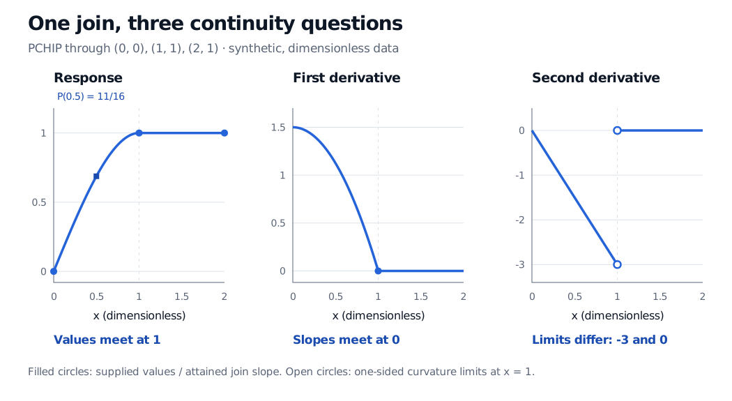
The secants are 1 and 0. PCHIP assigns slopes (m0,m1,m2)=(3/2,0,0) and produces
P(x)={23x−21x3,1,0≤x≤1,1≤x≤2.
Thus P(0.5)=11/16=0.6875 and P(1.5)=1. On the first interval, P′(x)=23(1−x2)≥0; on the second it is zero. The curve rises into the plateau without overshooting it.
At x=1, both pieces have value 1 and slope 0. Their second derivatives disagree:
x↑1limP′′(x)=−3,x↓1limP′′(x)=0.
PCHIP is therefore C1 here, but not C2: its first derivative is continuous, while the ordinary second derivative does not exist at this knot. A cubic spline with the usual simple-knot C2 conditions solves a different joining problem. Both are piecewise cubics; their slope choices and smoothness requirements differ.
Three panels show PCHIP through synthetic knots (0,0), (1,1), (2,1). The response joins at 1 and the first derivative joins at 0. At x=1 the second derivative has left limit -3 and right limit 0; open circles mark these limits.
Original synthetic example with dimensionless coordinates and responses. Matching values and slopes does not require matching curvature. Open circles in the last panel are one-sided limits, rather than an attained second derivative at the join.
Choose the interpolated quantity as well as the method
PCHIP can be useful when preserving the ordering of supplied values matters more than continuous curvature. Positive knot values also yield positive values between knots, because each interval stays within its endpoint range. These statements apply inside the knot domain. They do not establish a sensible extrapolation rule.
For a financial curve, specify whether the interpolated quantity is a discount factor, its logarithm, or a rate with a stated compounding convention. PCHIP's shape guarantee concerns that chosen quantity. It supplies no general convexity or financial no-arbitrage guarantee, and a quantity involving second derivatives may have jumps or be undefined at knots.
The Object-Oriented Model Design lesson (membership; public preview available) gives a useful implementation setting: its curve object interpolates log discount factors and rejects maturities outside its pillars. That example uses a different interpolation rule, but makes the choice of variable and domain explicit—the same decisions a PCHIP curve needs.
Gérard Cornuéjols, Javier Peña and Reha Tütüncü, Optimization Methods in Finance, 2nd edition, Cambridge University Press, 2018, §3.4, pp. 42–43 — interpolation between term-structure observations.