Construct a polynomial using cardinal weights, see why an interior weight can be negative, and distinguish exact interpolation from a suitable financial curve.
Lagrange interpolation
Lagrange interpolation writes the polynomial through supplied data points as a weighted sum of their values. Each weight is itself a polynomial chosen to select one input value at its own node and vanish at every other node.
For a quant filling gaps in a valuation grid, the attraction is exact agreement with the supplied results. The caveat is that the weights can be negative: an interpolated value need not behave like an average, and moving one input upward can move the answer downward.
Build a selector for each node
Given n+1 pairs (xj,yj) with distinct xj, define the cardinal basis polynomials
At x=xj, every factor in ℓj is one. At any other node xk, one factor is zero. Therefore pn(xj)=yj: the construction performs interpolation exactly in exact arithmetic.
The resulting polynomial has degree at mostn, rather than necessarily n. Collinear inputs, for example, produce a line even if more than two points are supplied. It is unique within this degree limit: the difference between two candidates would have n+1 distinct roots while having degree at most n, so it must be zero. This is the same unique curve that Newton interpolation expresses using divided differences.
Distinct nodes are essential. Two different values supplied at the same x cannot both be values of a single function. Repeating a node with the same value supplies no new constraint; it does not justify dividing by zero in the formula.
Three inputs, one negative weight
Take the synthetic, dimensionless points (0,1), (1,2) and (2,5). These might represent a small model-response grid; they are not market observations or interest rates. The basis functions are
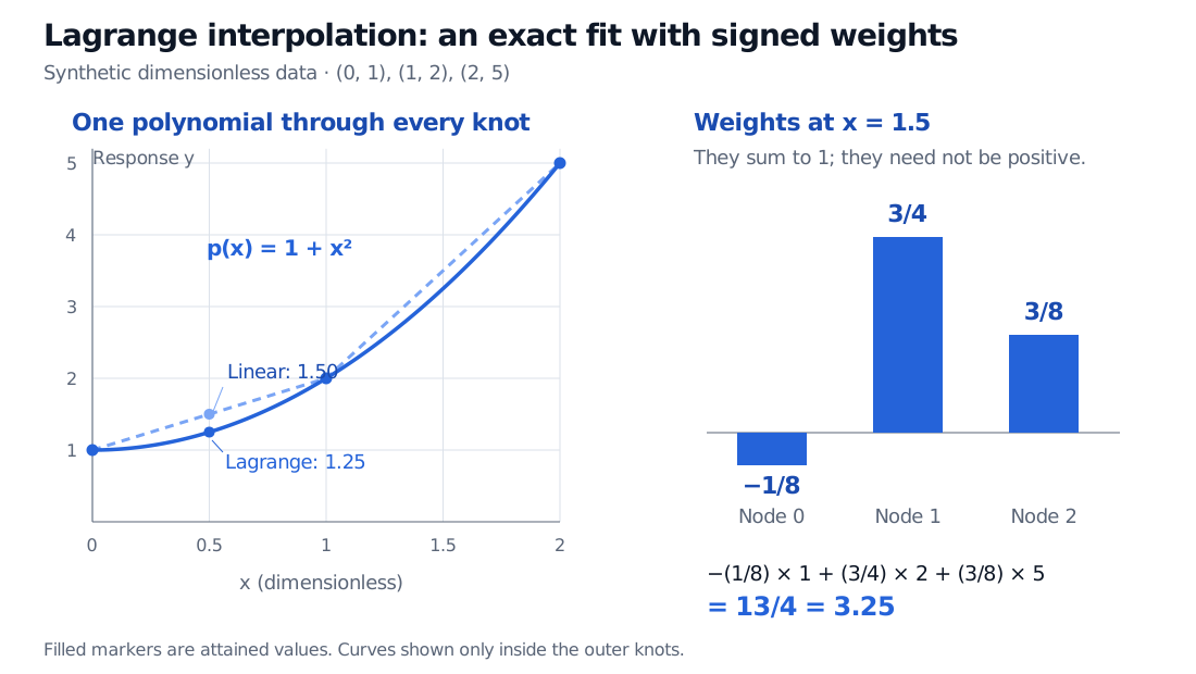
At x=1.5, the weights are −1/8, 3/4 and 3/8. They sum to one, but the first is negative:
p2(1.5)=−81×1+43×2+83×5=413=3.25.
At x=0.5, the polynomial gives 1.25. Piecewise linear interpolation between the first two nodes gives 1.50. Both methods fit all three nodes; they make different assumptions between them. Lagrange uses one polynomial across the whole grid, whereas the linear interpolant connects neighbouring points separately.
Through synthetic dimensionless points (0,1), (1,2) and (2,5), the Lagrange curve is 1+x squared. At x=0.5 it gives 1.25 versus 1.50 for piecewise linear interpolation. At x=1.5 its weights are minus 1/8, 3/4 and 3/8, producing 3.25.
Original synthetic example. The solid curve is the global quadratic; the dashed curve is piecewise linear. The separate bar chart shows signed weights at 1.5, not the contribution of each weighted response.
Read the weights as sensitivities
With the nodes fixed, changing an input value yj by Δyj changes the interpolated value by ℓj(x)Δyj. In this example, raising only the first response by 0.08 lowers the value at 1.5 by 0.01:
Δp2(1.5)=−81(0.08)=−0.01.
The identity ∑jℓj(x)=1 follows because interpolating constant data must reproduce that constant. It does not make these weights probabilities or long-only portfolio allocations.
A useful absolute sensitivity check is
∣Δpn(x)∣≤εj=0∑n∣ℓj(x)∣when∣Δyj∣≤ε.
At 1.5, the sum of absolute weights is 5/4=1.25. Thus bounded response errors can be amplified even inside the outer nodes. This is a fixed-node, absolute-error bound; it does not cover uncertainty in node positions or provide a relative-error bound near a zero response. Large weight sums warn about numerical conditioning, independently of whether the code fits the knots accurately.
Evaluate carefully; choose the curve deliberately
For computation, the barycentric form reuses weights depending only on the nodes:
At an exact node, return its supplied value directly: the displayed ratio has divisions by zero there, although the polynomial itself is well defined. The barycentric weights wj are distinct from the query-dependent cardinal weights ℓj(x). Multiplying all wj by the same nonzero constant leaves the ratio unchanged.
Barycentric evaluation avoids repeatedly expanding and evaluating the product formula. It does not remove poor node geometry, cure all rounding error, or stop high-degree global polynomials from oscillating. Reordering the same node/value pairs leaves the mathematical polynomial unchanged; finite-precision computations can differ. For many knots, a cubic spline offers a piecewise alternative whose boundary assumptions also need to be chosen.
In finance, choosing what to interpolate matters as much as fitting it. Interpolating zero rates, discount factors and log discount factors generally gives different intermediate valuations. SelfMadeQuant's Object-Oriented Model Design develops a discount-curve object using log-linear discount factors and an explicit maturity domain. The preview is public; the full lesson requires membership. It provides a useful concrete comparison with a global polynomial.
An exact knot fit alone establishes neither financial consistency nor an arbitrage-free yield curve. Nor does it justify extrapolation outside the supplied range. Those are separate modelling decisions and checks.
Rüdiger U. Seydel, Tools for Computational Finance, sixth edition, Springer, 2017, Appendix C.1, “Interpolation”, pp. 420–421: the Lagrange construction and piecewise alternatives to a high-degree global fit.