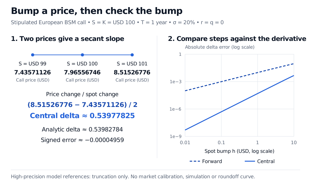
Estimate price sensitivities from bumped valuations, compare a call’s numerical and analytic delta, and separate truncation error from pricing noise and kinks.
Numerical differentiation
Numerical differentiation approximates a derivative using numerical evaluations of a function. In a pricing system, it lets a risk engine estimate a Greek by changing an input, repricing, and measuring the resulting slope. The pricer can be a closed-form formula, a simulation or a numerical solver; access to its symbolic derivative is unnecessary.
The useful question is not just “what slope did the calculation return?” It is “how sensitive is that slope to the bump, the pricing accuracy and what was held fixed?”
Choose the derivative before choosing the bump
Write V(S) for the value of one option, with strike, time remaining, volatility, rates and dividend yield held fixed. Its spot delta is the partial derivative∂V/∂S. A finite spot move produces a secant slope rather than the exact local derivative.
These orders require sufficient local smoothness—bounded second derivatives for the one-sided formulas and a bounded third derivative for the central formula. They describe truncation error as h tends to zero, before pricing and arithmetic errors. They do not guarantee a fixed number of correct digits.
The input convention matters. Bumping spot while keeping a model volatility fixed estimates a different sensitivity from bumping spot and recalibrating volatility. A volatility bump also needs a stated scale: a change of 0.01 in decimal volatility is one percentage point, not a one-percent relative change.
One call, three spot slopes
Consider a stipulated European call under the Black–Scholes–Merton model: spot and strike are both USD 100, time remaining is one year, volatility is 20% per square root of a year, and the continuously compounded risk-free rate and continuous dividend yield are both zero. This is a model calculation, not a market calibration. Prices are per option on one underlying unit, with no contract multiplier.
where Φ is the standard normal cumulative distribution function. The analytic result gives a benchmark for checking the numerical method.
With a USD 1 spot bump, the model prices are:
Spot (USD)
Call price (USD, rounded)
99
7.43571126
100
7.96556746
101
8.51526776
Using unrounded prices gives forward delta 0.54970030, backward delta 0.52985619, and central delta 0.53977825. Each is measured in USD of option value per USD of spot. For the central estimate,
2V(101)−V(99)≈0.53977825,
so its signed error, estimate minus analytic delta, is approximately −0.00004959.
For a stipulated BSM call, prices at spots USD 99, 100 and 101 are USD 7.43571126, 7.96556746 and 8.51526776. The USD 1 central bump gives delta 0.53977825 versus analytic delta 0.53982784. A log-scale comparison over spot bumps USD 0.01 to 10 shows the central truncation error below the forward truncation error in this example.
Original model calculation with fixed inputs. The curves use high-precision prices to isolate truncation error; they do not show market data, simulation noise or floating-point error.
Repeat the central calculation at smaller bumps:
Spot bump h (USD)
Central delta
Signed error
1
0.53977825
−0.00004959
0.5
0.53981543
−0.00001240
0.25
0.53982474
−0.00000310
The absolute error falls by almost a factor of four on each halving, consistent with second-order truncation here. This is a check of this smooth model and these steps, not a universal optimal bump rule.
The membership lesson Numerical Differentiation, which has a public preview, develops the formulas from Taylor expansions and compares bump-size effects.
What shrinking the bump can amplify
Suppose the two central-bump prices have additive evaluation errors e+ and e−. Before further arithmetic error, their contribution to the estimated delta is exactly
2he+−e−.
If each price error is bounded in absolute value by ε, this contribution is at most ε/h in magnitude. The finite-bump bias shrinks with h, but this worst-case bound grows. In floating-point arithmetic, subtracting nearby prices loses relative accuracy, and a sufficiently small intended bump can even round to the unchanged input.
Monte Carlo standard errors are uncertainty measures, not deterministic error bounds. If the two price estimators have standard errors s+ and s− and error covariance c, their central quotient has variance
4h2s+2+s−2−2c.
Common random numbers can help by making the pricing errors positively correlated. Check the uncertainty of the paired difference: two individually precise prices do not automatically give a precise small-bump Greek.
A stable quotient can still answer the wrong question
At expiry, the call payoff is g(S)=max(S−K,0). At S=K, every positive central bump gives
2hg(K+h)−g(K−h)=21.
The left derivative is zero and the right derivative is one. The classical derivative at the strike does not exist. An apparently perfect plateau across bump sizes therefore does not prove differentiability. This terminal payoff is distinct from the smooth, positive-time BSM price used above.
Finally, an analytic derivative differentiates a mathematical expression; automatic differentiation propagates derivatives through a program's operations using the chain rule. Finite differences estimate a slope from separated evaluations. They are different routes to sensitivities, and agreement is a useful check only when they target the same function, input convention and derivative.
Sources
John C. Hull, Options, Futures, and Other Derivatives, ninth Global Edition, Pearson, 2018, §19.4, pp. 424–426: delta as a price slope and the European call formula Φ(d1).