Estimate a derivative from the current and lower input values, check its first-order error, and distinguish a one-sided stencil from implicit time stepping.
Backward difference
A backward difference compares a function at the current input with its value one step lower. For a positive step h, the difference is f(x)−f(x−h); dividing by h gives the two-point approximation to the derivative:
Dh−f(x)=hf(x)−f(x−h).
For a quant computing a price sensitivity, this is useful when a lower bumped valuation is available but a higher input would leave the model's domain or the computed grid. “Backward” describes where the samples sit. It does not mean that the derivative is negative, or that the input must be calendar time.
A slope built from the left
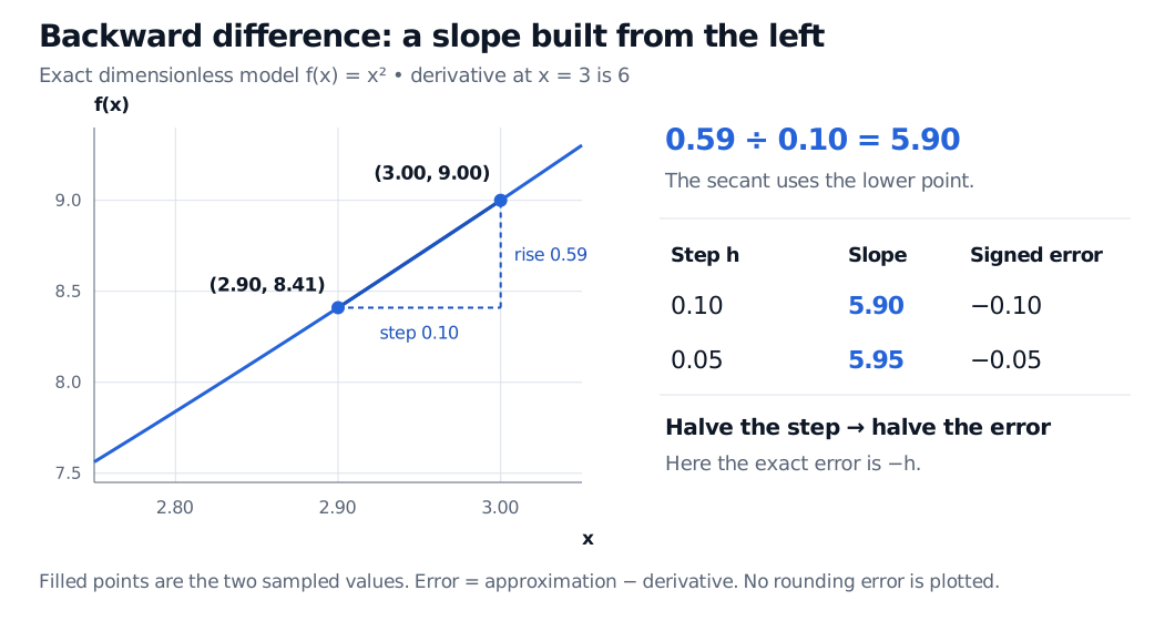
Take the dimensionless test function f(x)=x2 at x=3. Its exact derivative is f′(3)=6. With h=0.1, the two sampled values are f(3)=9 and f(2.9)=8.41, so
D0.1−f(3)=0.19−8.41=5.9.
The numerator is a function-value change of 0.59; the denominator is the positive input step of 0.1. Reversing the numerator while keeping this denominator would reverse the slope's sign.
Define signed error as approximation minus derivative. Here the entire error can be found algebraically:
Dh−f(3)=h9−(3−h)2=6−h,Dh−f(3)−6=−h.
Step h
Lower sample f(3−h)
Backward slope
Signed error
0.10
8.41
5.90
−0.10
0.05
8.7025
5.95
−0.05
Halving the step halves the error in this exact-arithmetic example. The secant joins the current point to a lower point on a convex curve, so its slope is below the tangent slope at the current point.
Exact dimensionless x-squared model: f(2.90)=8.41 and f(3)=9 give backward slope 0.59/0.10=5.90 versus derivative 6. Halving h to 0.05 gives 5.95 and halves signed error from minus 0.10 to minus 0.05.
Original exact-arithmetic example. The triangle separates the change in f from the positive input step; error means approximation minus derivative. No rounding error is plotted.
A forward difference instead samples 3+h and gives 6+h: it approaches from the other side. The central difference gives exactly 6 for this quadratic because its symmetric errors cancel. That exactness is a property of the quadratic, not a promise for every function.
Why the usual error is first order
If f is twice continuously differentiable on [x−h,x], Taylor's theorem gives
Dh−f(x)=f′(x)−2hf′′(ξ),x−h<ξ<x.
When ∣f′′∣≤M on the interval, the truncation error has magnitude at most Mh/2. With a uniform nearby bound as h→0, this is O(h): the two-point formula is first order. “Backward” itself does not specify an order; one-sided formulas using more sample points can achieve higher orders.
The quotient's units are always output units per input unit. If f is a value in USD and x is spot in USD per share, the slope is in shares. A price change without division by the spot step is not the same sensitivity.
What the stencil does not guarantee
A positive h must keep x−h inside the valid domain. At the upper endpoint of a computed grid, a backward stencil can use an existing interior node; near the lower endpoint, the same choice may be impossible. The domain decides which one-sided sample is admissible.
Making h smaller indefinitely can also damage the computed answer. Nearby inputs or function values can round to the same stored number, and subtracting nearby valuations can amplify rounding error. Check several steps in consistent units; a returned zero may reflect collapsed samples rather than a zero derivative.
Finally, a backward difference in a spatial input is a derivative stencil. Backward Euler is a time-stepping method: it couples a backward time difference with the differential equation evaluated at the new state. In option-pricing PDEs, that choice can require solving simultaneous equations. The word “backward” alone establishes neither implicitness nor stability. SelfMadeQuant's Finite Difference Methods lesson develops that connection; it has a public preview, with the full lesson available to members.
Sources
Seydel, R. U. (2017). Tools for Computational Finance, 6th edition. Springer. Sections 4.2.1, pp. 183–184, and 4.2.5, pp. 191–192: difference approximations and the implicit time scheme.
Driscoll, T. A. and Braun, R. J. Section 5.5: Convergence of finite differences. Truncation error and order. This article uses approximation minus derivative as its signed-error convention.
University of Illinois Urbana-Champaign, CS 357. Finite Difference Methods. The two-point backward derivative formula and its first-order truncation error.