Estimate parameters by matching theoretical and sample moments. Work an exponential arrival-rate example and see why support, identifiability and bias still matter.
Method of moments
The method of moments (MoM) estimates a model’s parameters by matching its theoretical moments to moments calculated from observed data, then solving the resulting equations. The simplest case matches a model’s expected value to the sample average.
It is a way to construct an estimator, rather than a guarantee that the estimate is unbiased, precise or a good description of the data. A desk might use it to obtain an initial arrival-rate estimate or starting values for a more demanding distribution fit.
From waiting times to an arrival rate
Suppose an execution researcher uses a deliberately simplified statistical model: four complete waiting times between comparable order arrivals are independent and identically distributed, with an exponential distribution and a constant unknown rate λ>0 per second. The synthetic observations are
x=(1,2,3,6) seconds.
In this rate parametrisation, EλX]=1/λ. The [sample mean is
xˉ=41+2+3+6=3 seconds.
Match the theoretical mean to the observed mean and solve:
λ^MoM1=xˉ⟹λ^MoM=xˉ1=31 per second.
The fitted mean wait is three seconds. The rate has inverse-time units; three seconds is not the estimated rate. This calculation also equals the maximum likelihood estimate for these complete IID exponential observations. That agreement is a property of this model, not an equivalence between the two estimation methods.
The example assumes exact recorded durations. In real order data, changing activity, clustered arrivals, timestamp rounding and waits cut off by the observation window can change the appropriate model and estimation equations. A reciprocal sample mean does not establish that exponential waiting times are a good fit.
What equations are being solved?
For a parameter vector θ, a raw population moment and its sample counterpart are
mj(θ)=Eθ[Xj],m^j=n1i=1∑nXij.
An ordinary MoM construction selects moments and solves mj(θ^)=m^j. For two unknown parameters, one often uses the first two raw moments. The second raw moment is not the variance: Var(X)=m2−m12. Matching these two moments therefore produces the variance expression m^2−m^12, with divisor n, rather than automatically applying an unbiasedness correction.
Three checks matter before accepting a solution:
The moments must exist. A finite sample always has computable powers, but the corresponding population expectations may be undefined or infinite. A sample average cannot supply a missing theoretical mean.
The selected moments must identify the parameters. Counting equations is insufficient. For example, the mean of a zero-mean normal model is zero for every positive variance: its first moment contains no information that distinguishes those variances. The second moment does. This is identifiability through the chosen moment map.
The equations must have an acceptable solution. A nonlinear system can require numerical root finding, have several roots or have no root in the parameter space. Closed-form algebra is convenient when available; it is not part of the definition.
Extra sample moment equations are generally not redundant. In the exponential example, the sample second raw moment is 12.5 seconds2, whereas the fitted model’s second moment is 2/λ^2=18 seconds2. The first-moment fit cannot match both. With more moment restrictions than parameters, generalised method of moments provides a framework for choosing a weighted compromise, subject to its own identification and sampling conditions.
A valid parameter can still exclude an observation
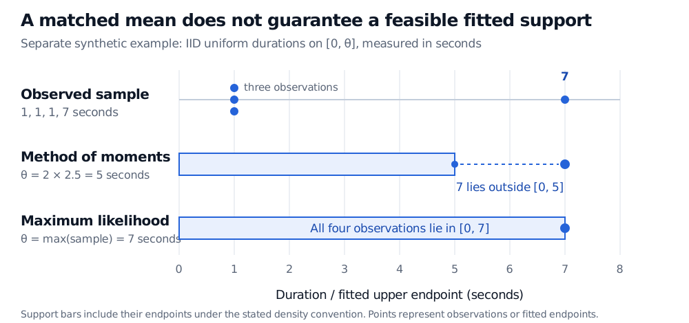
Consider a separate synthetic example: durations modelled as uniform on [0,θ], where θ>0 seconds. Its mean is θ/2. For observations (1,1,1,7) seconds, the sample mean is 2.5 seconds, giving
θ^MoM=2xˉ=5 seconds.
Five is an allowed positive parameter, but the fitted interval [0,5] excludes the observed duration of seven seconds. Matching a mean has ignored information about the sample’s maximum.
For a separate synthetic sample of 1, 1, 1 and 7 seconds, uniform moment matching gives upper endpoint 5 seconds, excluding the 7-second observation. Maximum likelihood with inclusive endpoints gives 7 seconds, containing all four observations.
The bars show fitted uniform supports, not confidence intervals. Repeated observations at one second are stacked. Both calculations use the same separate synthetic sample.
Using the density convention f(x;θ)=1/θ for 0≤x≤θ and zero otherwise, the likelihood is zero when θ<7 and decreases as θ−4 when θ≥7. The MLE is therefore seven seconds. With a strictly open upper endpoint in the chosen density version, no maximum is attained: the likelihood supremum is approached as θ decreases to seven from above. The boundary convention must be stated. This example demonstrates a support conflict, not evidence that real waiting times follow a uniform law.
Matching a mean does not preserve unbiasedness
Under the IID exponential model, Xˉ is unbiased for 1/λ. Taking its reciprocal does not preserve that property. If S=∑iXi, then S has a gamma distribution with shape n and rate λ, so
Eλ[λ^MoM]=nEλ[S1]=n−1nλ,n>1.
The estimator is upward biased; at n=4, its repeated-sampling expectation is 4λ/3. The true λ is unknown, so this does not tell us the error in the particular estimate 1/3. Under this model, (n−1)/S is an unbiased estimator of the rate, giving 1/4 per second for the observed data. That adjustment serves a different criterion from matching the sample mean.
MoM can nevertheless be consistent. Under IID sampling, finite absolute moments give convergence of the selected sample moments by the law of large numbers. If an appropriate inverse moment map exists and is continuous at the true moments, the fitted parameters converge to their true values. This large-sample statement does not remove finite-sample bias, establish efficiency or validate the assumed model.
For a fuller comparison of estimator bias, mean squared error and likelihood fitting, see Estimation and Maximum Likelihood (membership; public preview).
Sources
John A. Rice, Mathematical Statistics and Data Analysis, 3rd ed., §8.4, “The Method of Moments”: moment inversion, examples and consistency.
George Casella and Roger L. Berger, Statistical Inference, 2nd ed., §7.2.1: construction of moment estimators and parameter-space failures.
Yen-Chi Chen, University of Washington, STAT 512, Lecture 6: Estimators, “Method of moments estimator” and the uniform maximum-likelihood example.