A statistical model is a family of possible data laws. Separate assumptions from a fitted member using a normal-return example, likelihood comparison and explicit units.
Statistical model
A statistical model is a family of possible probability laws for observed data, together with the sampling or dependence structure those laws impose. It describes what could generate the observations and which features remain unknown. A fitted model selects a member of that family using data; it does not establish that the family is appropriate.
For a quant estimating daily return risk, “returns are normal” is incomplete. Are returns independent across days? Does their distribution stay the same? Are the observations daily log returns, simple returns, or overlapping five-day returns? Those choices change the data law and the uncertainty of an estimate, even if the same bell curve is drawn for a single observation.
The family comes before the fit
Write the entire observed sample as X=(X1,…,Xn). A model can be written
P={Pθ:θ∈Θ}.
Here Pθ is a probability distribution for the whole sample, and Θ contains the allowed values of the parameter or parameter vector. Before observation, X is random; afterwards, the realised values x are fixed data.
For example, suppose one-period log returns are independent and identically distributed, with
Xi∼N(μ,σ2),μ∈R,σ>0.
This is an IID normal model. Normality specifies the shape of each one-period distribution; independence specifies how observations combine; identical distribution holds the parameters constant across periods. The joint density is therefore a product:
fμ,σ(x1,…,xn)=i=1∏nσ2π1exp[−2σ2(xi−μ)2].
The product does not follow from normal marginals alone. Correlated normal observations can have the same marginal means and variances but a different joint law. In a financial time series, dependence or changing conditional volatility can matter as much as the marginal distribution.
Three returns, two unknown parameters
Consider an original synthetic sample of daily log returns: −1%, 0%, +1%. Record returns in percentage points (pp), so the numerical data are x=(−1,0,1), not (−0.01,0,0.01). Under the IID normal model, maximum likelihood estimation gives
μ^=xˉ=0 pp,σ^2=31i=1∑3(xi−xˉ)2=32 pp2.
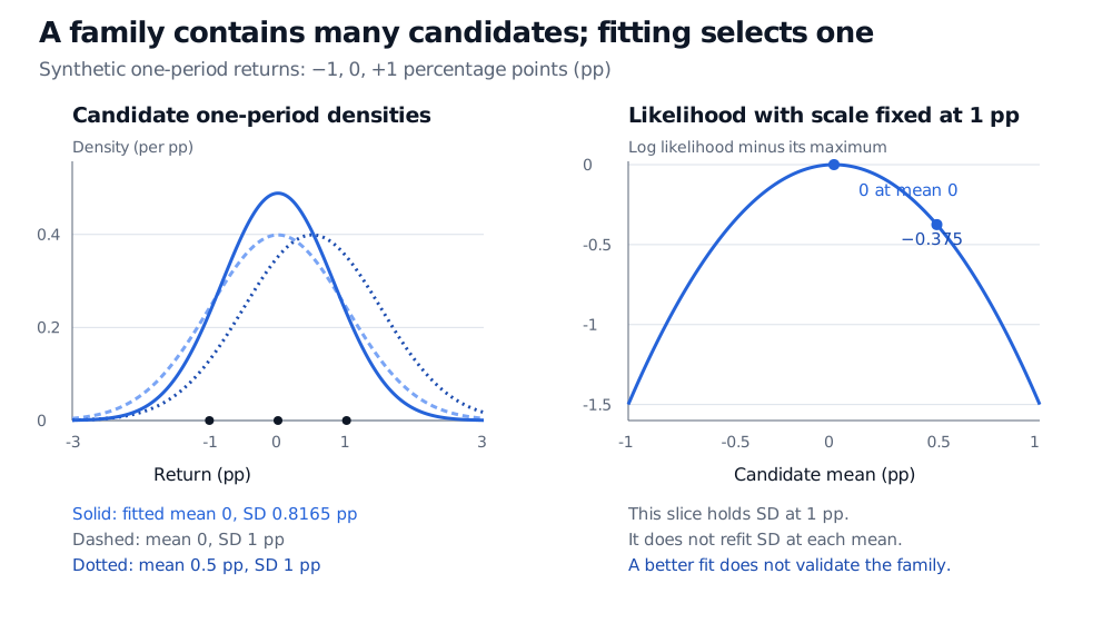
The fitted standard deviation is approximately 0.8165 pp. The divisor is three because this is the normal maximum-likelihood variance estimate; the familiar unbiased sample variance uses n−1 and would equal 1 pp2 here. These answer different estimation questions.
The fitted one-period distribution is N(0,2/3) when returns are measured in pp. The model remains the entire IID normal family. Three observations do not prove normal tails, independence, or stable parameters, and a fitted mean of zero does not establish that the population mean is zero.
Synthetic returns −1, 0 and +1 pp. Left: three candidate normal densities, including the fitted mean 0 and standard deviation 0.8165 pp. Right: at fixed standard deviation 1 pp, relative log likelihood peaks at mean 0 and equals −0.375 at mean 0.5 pp.
Original synthetic illustration. The left panel shows individual-observation densities; the right uses all three observations and holds standard deviation fixed at 1 pp. Dots on the left baseline mark observed returns, not probability masses.
What the likelihood actually compares
A likelihood holds the observed sample fixed and varies the candidate parameters. To isolate the mean comparison, fixσ=1 pp instead of using its fitted value. In these numerical units,
where C is constant in μ. The mean-zero candidate has about 1.455 times the likelihood of the mean-0.5 candidate. This compares two members of a specified family; it is neither the probability that the first mean is true nor evidence that the whole normal family is correct.
For continuous returns, a density value is not the probability of observing that exact return: an exact point has probability zero. A one-period density measured on the pp scale has units per pp; the three-observation joint density has units per pp cubed. Probabilities come from integrating over intervals. Changing to decimal returns multiplies each density by 100, and this joint likelihood by 1003; the likelihood ratio above is unchanged. Absolute likelihood values require a consistent data scale and reference measure.
Assumptions survive optimisation
Before using a fitted law for a tail-loss calculation, ask whether its restrictions address the decision. Normal fitting cannot introduce heavy tails that the family excludes. IID fitting cannot learn volatility clustering while retaining independence and a constant variance. Such failures are model risk, distinct from uncertainty about parameters within the chosen family. Inspecting residuals, dependence and tail behaviour, checking stability across periods, and evaluating later observations address different parts of that risk; none certifies a model as universally valid.
The normal example is parametric: a fixed finite-dimensional vector describes the unknown distribution. More flexible, nonparametric models can leave an entire distribution or function unknown, often subject to smoothness or shape restrictions. “Nonparametric” does not mean assumption-free: sampling, dependence and regularity conditions still determine what inference is justified. Greater flexibility can reduce one kind of misspecification while making estimation harder with limited data.
For a deeper treatment, Parametric Statistical Models and the Likelihood develops parameter spaces, identifiability and the likelihood distinction. The public page is a preview; the complete lesson requires membership.
Sources
Larry Wasserman, All of Statistics: A Concise Course in Statistical Inference, Springer, §6.2 (parametric and nonparametric models), §9.3, especially Example 9.11 (normal maximum likelihood), and §9.12 (checking assumptions).