Mean squared error averages squared mistakes. Compare estimator risk with forecast MSE, and see when a biased fill-probability estimate improves the score.
Mean squared error
Mean squared error (MSE) is the average of squared errors. For an estimatorθ^ of a fixed parameter θ, it is the repeated-sampling quantity
MSEθ(θ^)=Eθ[(θ^−θ)2].
The expectation averages over the data that could have been observed under the model with that same θ. It does not average over possible parameter values. In quant finance, MSE helps compare noisy estimates of fill probabilities, expected returns or model coefficients: a rule that moves estimates away from their raw values can still reduce average squared error.
The distinction is practical. A smaller MSE describes a better average score under a specified model and loss; it does not promise a smaller error on the next dataset.
Two ways an estimate misses
With finite second moments, MSE separates into variance around the estimator's own mean and squared bias away from the target:
MSEθ(θ^)=Varθ(θ^)+(Eθ[θ^]−θ)2.
To see why, write the error as
θ^−θ=(θ^−Eθ[θ^])+(Eθ[θ^]−θ).
Squaring and taking expectations kills the cross term: the first bracket has mean zero. An unbiased estimator therefore has MSE equal to its variance. A biased one must pay for its squared bias, but a large enough reduction in variance can more than cover that cost.
Four orders, two rules
Consider a deliberately small execution model: four comparable orders have independent fill indicators, each with the same unknown fill probability p. Then the number filled is K∼Binomial(4,p), a binomial distribution. These are stipulated assumptions, not claims about actual order dependence.
Compare the raw fill fraction with a smoothed rule:
p^raw=4K,p^smooth=6K+1=32p^raw+31(21).
The second rule pulls the raw fraction toward one half. Its extra success and failure are a smoothing convention, not two additional observed orders.
For this calculation, suppose the model's true p is 1/4. Across repeated batches of four orders:
Quantity
Raw K/4
Smoothed (K+1)/6
Expected estimate
1/4
1/3
Bias
0
1/12
Variance
3/64
1/48
Squared bias
0
1/144
MSE
3/64=0.046875
1/36≈0.027778
The smoothed estimator is biased upward here, yet has lower MSE because
481+1441=361<643.
That is an average over the sampling distribution, not a verdict on every outcome. If exactly one order fills, the raw estimate equals the stipulated truth 1/4, while the smoothed estimate is 1/3. On that batch, raw has zero error and smoothing makes it worse.
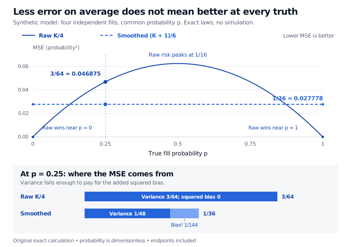
Exact risk curves for four iid Bernoulli orders: raw K/4 has MSE p(1-p)/4 and smoothing (K+1)/6 has constant MSE 1/36. At p=0.25 raw MSE is 3/64, while smoothing combines variance 1/48 and squared bias 1/144. Raw wins near p=0 and p=1.
Original exact model calculation. Probabilities are dimensionless; the plotted score is squared probability error. The lower bars split the score at p=0.25 into variance and squared bias.
Changing the unknown truth changes the comparison. For arbitrary p∈[0,1] in this same four-order model,
At p=0, the raw estimate is always correct, so its MSE is zero; smoothing always reports 1/6, giving MSE 1/36. The same disadvantage occurs at p=1. Smoothing wins between the two risk-curve crossings, approximately 0.127 and 0.873, and loses outside them. Neither of these two rules uniformly dominates the other. Constant risk is a property of this particular smoothing rule with four observations, not a general promise about adding one success and one failure.
For the broader estimation framework, Estimation and Maximum Likelihood develops the bias–variance identity and Bernoulli estimator alongside likelihood methods. The public page is a preview; the full lesson requires membership.
When “MSE” is a forecast score
In prediction work, the same name commonly means an empirical average over observed outcomes yi and their forecasts y^i:
MSEprediction=m1i=1∑m(yi−y^i)2.
Here the averaging is over the m evaluation cases actually recorded, rather than every possible sample at a fixed unknown parameter. The denominator is the number of scored cases, not a degrees-of-freedom correction for estimating a noise variance. This is the standard prediction-metric convention.
For example, three synthetic slippage forecasts of 1 basis point each face realised slippage of 0, 3 and −2 basis points. Their squared errors are 1, 4 and 9 basis points squared, so empirical MSE is 14/3 basis points squared. Its square root, RMSE, is approximately 2.16 basis points. MSE has squared units; RMSE restores the target's units.
A forecast score on genuinely held-out, appropriately timed observations can help assess future prediction risk. It is still a finite-sample measurement, and noisy future outcomes contribute error even when their conditional mean is predicted correctly. Training MSE is especially easy to improve through overfitting. For the distinction between empirical risk, population risk and held-out evaluation, see The Supervised Learning Problem and the ML Pipeline, also available as a public preview with the full lesson requiring membership.
Choose what an error should cost
MSE is expected loss under squared-error loss: L(θ,a)=(a−θ)2. It penalises an error twice as large four times as much, and treats equally sized overestimates and underestimates identically.
Those choices need to suit the decision. If understating trading costs is more damaging than overstating them, a symmetric score may hide the distinction that matters. Squared prediction loss targets a conditional mean; a median or a tail quantile calls for a loss suited to that target. Nor does low MSE establish representative data, stable market conditions or profitable trades. It answers a precise scoring question, whose target, units, sampling assumptions and consequences must be stated.
Sources
George Casella and Roger L. Berger, Statistical Inference, second edition, Duxbury, 2002, §7.3.1, definitions 7.3.1–7.3.2, pp. 330–332; §7.3.4, loss and risk functions, pp. 348–350.