Local volatility makes instantaneous return volatility a fixed function of stock price and time. Understand its random path, Dupire calibration and limits for exotic pricing.
Local volatility
Local volatility is an asset's instantaneous return-volatility coefficient specified as a deterministic function of the current asset price and time. It extends the Black–Scholes model by replacing one constant volatility with a rule σloc(t,S). A derivatives desk can use such a rule to price different payoffs within one model, while calibrating the rule to today's European option prices.
The rule is deterministic; the future stock price is random. Consequently, the volatility experienced along a future stock path is generally random too. “Deterministic volatility function” does not mean that tomorrow's volatility is known today.
Here St>0 is the stock price, r(t) and q(t) are deterministic continuously compounded interest and proportional dividend-yield rates, and Wt is Brownian motion under that measure. Time is measured in years. Volatility has units of inverse square-root years; a numerical annualised volatility of 0.20 is conventionally quoted as 20%.
Imagine a hypothetical model in which lower stock prices lead to higher local volatility. Let s denote the numerical stock price in USD per share, and specify the numerical annualised volatility as
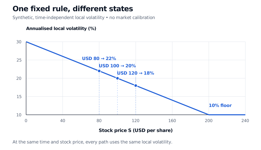
σloc(t,s)=min(0.40,max(0.10,0.20+0.001(100−s))).
The coefficient 0.001 is tied to the USD price scale: changing the currency or quoting shares in cents requires changing the rule. There is no explicit time dependence in this particular example; it is a special case of a time-and-state function.
Stock price, USD per share
Local volatility, annualised
Instantaneous return-variance rate, per year
80
22%
0.0484
100
20%
0.0400
120
18%
0.0324
Suppose two paths reach USD 80 and USD 120 at the same future time. They use 22% and 18% volatility respectively. If those paths later meet at the same price and time, they use the same volatility there, regardless of how they arrived. No additional variance state is needed to make that lookup.
Synthetic local-volatility rule decreases from 30% at USD 0 to a 10% floor at USD 200. At stock prices USD 80, USD 100 and USD 120, annualised local volatility is 22%, 20% and 18%.
Original synthetic state rule, with time measured in years and stock prices in USD per share. The 10% floor starts at USD 200. For nonnegative stock prices the rule never reaches its 40% upper cap. This is not a fitted market surface.
At USD 80, 0.222=0.0484 is a variance rate. Over an infinitesimal interval dt, the conditional log-return variance has leading term 0.0484dt. It is not a claim that the next year's log-return variance is 0.0484: the stock can move, changing the volatility it experiences. The quadratic variation of log price accumulates as
[logS]T=∫0Tσloc2(t,St)dt.
That path integral is generally random. A historical realised-volatility estimate is a separate statistic computed from observed returns.
Local volatility and implied volatility answer different questions
Implied volatility is the constant Black–Scholes input that reproduces a particular option price. Its surface is indexed by strike and expiry, given today's spot and valuation date. Local volatility specifies the instantaneous movement of the underlying at a time and asset-price state.
A local-volatility model produces option prices; those prices can then be inverted into an implied-volatility surface. The two surfaces are not generally equal point by point. In particular, the synthetic value σloc(t,80)=22% does not imply that every option struck at USD 80 has 22% implied volatility.
Dupire's formula connects the objects through derivatives of call prices. To see the central mechanism without carry adjustments, assume zero interest and dividend yield. If C(K,T) is today's European call price at strike K and expiry T, then
σloc2(T,K)=K2∂2C/∂K22∂C/∂T.
This classical expression needs a sufficiently smooth call-price surface: once differentiable in maturity and twice in strike, with positive strike curvature where the ratio is evaluated. It also requires consistent European contract and carry conventions, appropriate boundary conditions, a nonnegative variance ratio, and coefficients admitting a well-defined diffusion. An ideal, complete, arbitrage-consistent surface satisfying the needed conditions can be reproduced by the resulting diffusion. A finite, noisy quote grid does not automatically provide those conditions.
The strike derivative measures curvature related to the risk-neutral density. Differentiating sparse quotes amplifies noise; smoothing and extrapolation can materially affect the extracted local volatility. Where the curvature vanishes, the displayed division cannot identify a finite coefficient. With nonzero carry, use the carry-adjusted formula rather than the zero-carry version above. Columbia's model-risk notes give that version and discuss the calibration difficulties.
For the forward PDE and its carry terms, read §1.1–1.2 of The Dupire PDE and the Local Vol Formula. The public page is a preview; the full lesson requires membership.
A good fit today leaves a dynamics choice
A stochastic-volatility model such as Heston introduces a separate variance state with its own dynamics. Its Brownian driver may be correlated with the stock-price driver; “separate” does not mean statistically independent. At the same time and stock price, different Heston paths can still have different instantaneous variances. Pure local volatility rules that possibility out.
Matching today's European calls constrains the distribution of the stock at each expiry. It does not uniquely determine how the stock travels between dates. Models can therefore agree on vanilla prices while disagreeing on barrier-option values, future smiles and hedging behaviour. Gatheral develops this distinction in Chapters 1 and 8: a local-volatility fit is a consistent pricing construction under its assumptions, not proof that its future volatility dynamics describe the market.
Sources
John C. Hull, Options, Futures, and Other Derivatives, 9th Global Edition, §27.3, “The IVF Model,” equation 27.4 — state-and-time volatility, carry-adjusted extraction and practical smoothing.
Jim Gatheral, The Volatility Surface: A Practitioner's Guide (Wiley, 2006), Chapter 1, “Local Volatility,” pp. 7–11; Chapter 8, “Dynamics of the Volatility Surface” — local-volatility construction and the limitations of its implied dynamics.