A homogeneous Poisson process has a constant arrival rate and independent stationary increments. See why three arrivals per hour does not mean one every twenty minutes.
Homogeneous Poisson process
A homogeneous Poisson process counts random arrivals at a constant rate, with independent counts in disjoint time intervals. “Homogeneous” means that shifting a window along the time axis does not change its count distribution. It does not mean one arrival at regular intervals.
That distinction matters when a quant models claim notifications, operational incidents or price-jump times. A rate of three arrivals per hour can give useful probabilities for a quiet window or a burst of activity. It does not promise one arrival every twenty minutes, and a fitted hourly average alone does not establish the model's independence assumptions.
What stays the same when the clock moves
Let Nt count arrivals in (0,t], with N0=0. For a constant rate λ>0, the count in any window of duration h≥0 has a Poisson distribution:
Ns+h−Ns∼Poisson(λh),s≥0.
The standard process has right-continuous paths that jump upward by one at each arrival. Two properties govern how its windows fit together:
Stationary increments: the distribution above depends on h, not the starting time s. Every twenty-minute window has the same count probabilities.
Independent increments: counts in non-overlapping windows are independent. An unusually busy first window does not change the next window's distribution under the model.
Stationary increments do not make the cumulative count stationary. Its expectation grows as E[Nt]=λt. Independence applies to separate window counts, not to overlapping totals such as N20 and N40 when time is measured in minutes.
The broader label Poisson process often means this constant-rate model unless a varying intensity is specified.
Three per hour: count a window or wait for one arrival
Suppose a hypothetical monitoring service models incident notifications at 3 per hour. This is a synthetic timing model, not an estimate from operational or market data.
For a 20-minute window, rate and duration must use matching units:
λh=3hourarrivals×31hour=1arrival.
The expected count is one, and the count variance is numerically one, in squared-count units. Neither says the realised count must equal one.
Question
Model calculation
Probability
No notifications in twenty minutes?
e−1
36.79%
At least one in twenty minutes?
1−e−1
63.21%
Exactly two in one hour?
e−332/2!
22.40%
The third question uses mean count three because its window is a full hour. In particular, λh is an expected count, not an exact arrival probability.
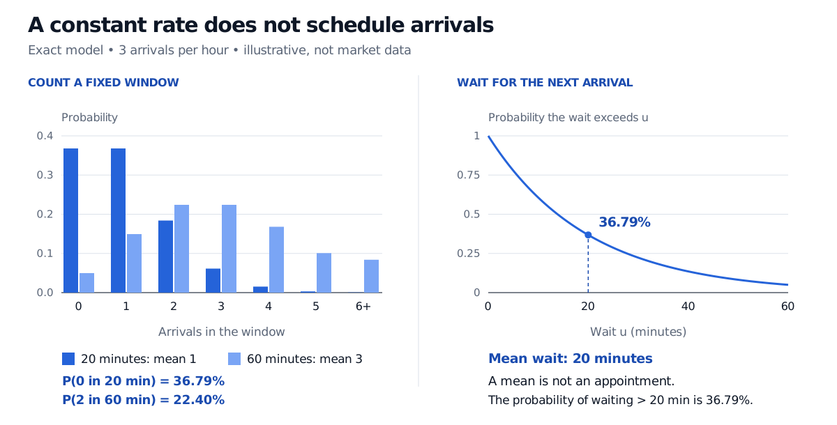
Exact rate-three-per-hour model. Twenty-minute counts have mean one and probability zero 36.79%; hourly counts have mean three and probability two 22.40%. The next-arrival waiting-time survival curve is exponential, with probability 36.79% of exceeding the mean wait of twenty minutes.
Original exact model, with no simulated or empirical data. Left: changing the window changes the Poisson mean; the final bar includes all counts of six or more. Right: a twenty-minute mean wait still leaves a 36.79% chance of waiting longer.
The same process can be built from independent, identically distributed exponential waiting times. If W is the wait from a fixed observation time to the next arrival, then
P(W>u)=e−λu,E[W]=λ1.
Here 1/λ=1/3 hour, or 20 minutes. The identical formula for P(W>20 minutes) and the zero-count probability is no coincidence: waiting longer than the window means observing no arrivals inside it.
After twenty minutes with no notification, the expected additional wait remains twenty minutes. The exponential clock is memoryless; an arrival has not become “due.” The independent-clock construction and fresh-start property are developed in Defining the Poisson Process: Three Equivalent Constructions, available with membership and a public preview.
Which assumption needs changing?
Predictably busier hours call for a deterministic time-varying rate. Counts can still have independent increments, but their mean becomes the integrated rate over each window, and equal-length windows need not have identical distributions. MIT's Poisson-process notes, §2.4 explain this non-homogeneous extension.
If arrivals themselves trigger further arrivals, timing dependence is a separate issue; a Hawkes process can model self-excitation. If the missing ingredient is the financial size attached to each arrival, a compound Poisson process adds marks or jump sizes. Homogeneity concerns the arrival rate, not identical loss amounts.
The zero-rate boundary is also simple: every finite-window count is zero, and there is no finite next-arrival time. A zero-length window contains no arrivals for any finite rate.
Sources
Richard Durrett, Essentials of Stochastic Processes, third edition, Springer, 2016, Chapter 2, §§2.1–2.2.2 — exponential clocks, Poisson count moments, independent stationary increments and limitations of constant intensity.