Independent increments: Definition & Examples

A process has independent increments when its changes over disjoint time intervals are jointly independent. Learning the realised change in one of those intervals does not alter the probability law of the changes in the others. This assumption makes it possible to simulate a price model's underlying shocks one time step at a time using fresh random draws.

The interval boundaries matter. Even when the underlying shocks have independent increments, two overlapping return windows can depend on each other because they include some of the same shocks. Treating rolling observations as independent can therefore overstate how much information a sample contains.

What the assumption actually says

For a stochastic process

X_t

and any deterministic times

0\le t_0<t_1<\cdots<t_n,

the random variables

X_{t_1}-X_{t_0},\quad X_{t_2}-X_{t_1},\quad\ldots,\quad X_{t_n}-X_{t_{n-1}}

must be jointly independent, for every finite choice of the times. Merely checking every pair is weaker than checking joint independence of the whole collection. The equivalent disjoint-interval formulation also permits gaps between the intervals. Lalley's Brownian-motion notes, §2 state this distinction from stationary increments explicitly.

For Brownian motion relative to an information flow

\mathcal{F}_t

, one additionally specifies that

W_t-W_s

is independent of

\mathcal{F}_s

for

s<t

. With the natural information flow,

\mathcal{F}_s

records the path through time

s

. An enlarged information set must satisfy this condition too: if it reveals a future shock, the condition fails. “Independent of the past” is therefore a statement about a stated model and information set, not a conclusion about actual market efficiency.

Adjacent shocks, overlapping windows

Take standard Brownian motion and measure time in years. Its increment over $(s,t]$ has distribution $\mathcal{N}(0,t-s)$ , with variance measured in years under this normalization.

The adjacent changes

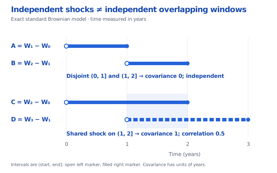
A=W_1-W_0,\qquad B=W_2-W_1

are independent, each with distribution $\mathcal{N}(0,1)$ . Sharing the boundary time 1 does not create overlap: the half-open intervals $(0,1]$ and $(1,2]$ are disjoint.

Now make the windows longer:

C=W_2-W_0,\qquad D=W_3-W_1.

Write $Z_1=W_1-W_0$ , $Z_2=W_2-W_1$ and $Z_3=W_3-W_2$ . These three unit-year shocks are independent standard normals. But $C=Z_1+Z_2$ and $D=Z_2+Z_3$ both contain $Z_2$ . Consequently,

\begin{aligned} \text{Var}(C)&=\text{Var}(D)=2,\\ \text{Cov}(C,D)&=\text{Var}(Z_2)=1,\\ \text{Corr}(C,D)&=\frac{1}{\sqrt{2\cdot2}}=0.5. \end{aligned}

Brownian interval diagram: adjacent unit-year increments are independent; overlapping two-year increments share one year of shocks and have correlation 0.5.

Original exact Brownian model. Adjacent half-open intervals share no time; the longer windows share the shock on $(1,2]$ . Each longer increment has variance 2 years, so one year of shared variance gives correlation 0.5.

For forward Brownian increments over arbitrary intervals, the covariance is the length of their overlap:

\text{Cov}(W_b-W_a,W_d-W_c) =\max\{0,\min(b,d)-\max(a,c)\}, \qquad a\le b,\ c\le d.

This follows by expanding the four terms using

\text{Cov}(W_s,W_t)=\min(s,t)

. Notice also that the levels

W_1

and

W_2

are dependent: their covariance is 1. Independent increments do not mean independent process values.

The simulation formula and level covariance are developed further in SelfMadeQuant's Stochastic Processes, Brownian Motion and Itô's Lemma, Definition 3.2 and Proposition 3.3. The link opens a public lesson preview; the full lesson requires membership.

Independence and stationarity answer different questions

Stationary increments say that an increment's distribution depends on the interval's length, rather than its position in time. Independence says how increments relate to one another. Neither condition implies the other.

Model	Independent increments?	Stationary increments?
Standard Brownian motion	Yes	Yes
Non-homogeneous Poisson process with deterministic increasing rate	Yes	Generally no
$X_t=tZ$ , with one shared $Z\sim\mathcal{N}(0,1)$	No	Yes

For the counting example, let

t

be the numerical number of hours since a specified opening time and let the deterministic rate be

\lambda(t)=2t

events per hour for

t\ge0

. In this non-homogeneous Poisson process, counts over disjoint intervals remain independent. Their means, however, differ:

\mathbb{E}[N_1-N_0]=\int_0^1 2u\,du=1, \qquad \mathbb{E}[N_2-N_1]=\int_1^2 2u\,du=3.

These are independent Poisson counts with parameters 1 and 3. The same one-hour duration does not give the same law. A busier later hour reflects the deterministic schedule, without making an earlier count informative about the later count. The integrated-intensity and deterministic time-change constructions appear in Gallager's MIT notes, §2.4.

In the common-factor example, $X_{s+h}-X_s=hZ$ , which has the same law for every starting time $s$ . Yet adjacent unit-time increments both equal $Z$ . Observing the first reveals the second exactly; their covariance and correlation are both 1. Stationarity has preserved the distribution while leaving complete dependence.

Why zero correlation is an incomplete check

Independent finite-variance increments have zero covariance, but the reverse implication needs extra structure. For a jointly Gaussian vector of increments, a diagonal covariance matrix does imply joint independence. Normal marginal distributions alone do not establish joint Gaussianity.

For example, let

U=Z

and

V=SZ

, where

Z

is standard normal and

S

is an independent fair random sign. Both

U

and

V

are standard normal and their covariance is zero. Nevertheless,

|U|=|V|

always, so they are dependent. A correlation estimate near zero cannot establish independent market shocks or validate an independent-increment model by itself.

Sources

Steven Lalley, Lecture 5: Brownian Motion, University of Chicago, §2: independent and stationary increment definitions.
Robert G. Gallager, Discrete Stochastic Processes, Chapter 2: Poisson Processes, MIT OpenCourseWare, §2.4: non-homogeneous Poisson processes and integrated intensity.
Gregory F. Lawler, Stochastic Calculus: An Introduction with Applications, revised 15 February 2023, §§2.4, 2.6.1 and 2.6.3: Brownian increments, information flows and Gaussian covariance structure.

What the assumption actually says

Adjacent shocks, overlapping windows

Independence and stationarity answer different questions

Why zero correlation is an incomplete check

Sources

Related terms

Brownian motion

Correlation

Covariance

Independence

Poisson process

Stationary increments

Stochastic process