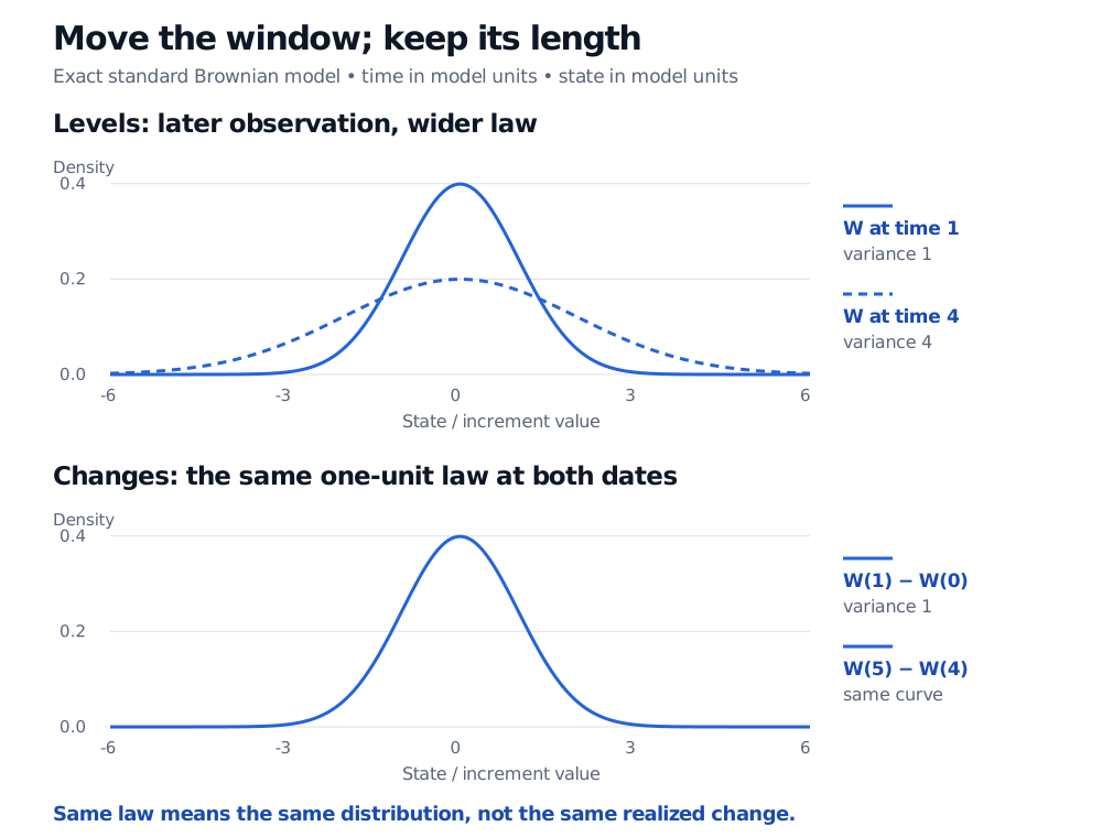
Slide a fixed-length observation window: its change can keep the same law even as the process level spreads out. Distinguish marginal and joint conventions.
Stationary increments
Stationary increments mean that the distribution of a process's change over an interval depends on the interval's length, rather than its starting date. In a simulation model, that lets the same one-day shock law serve a window starting today or a window starting later. It does not say that the process's level has a stable distribution.
The symbol =d means equality in distribution. The two random changes need not have the same realized value. Keeping h fixed is essential: changing the window's length is a different operation from sliding it along the time axis.
Slide a Brownian window
Let Wt be standard Brownian motion, with time and state expressed in model units. Look first at its levels:
W1∼N(0,1),W4∼N(0,4).
The second parameter is the variance. Standard deviations are therefore 1 and 2. These distributions differ, so the process is not stationary in levels. Now measure a change over a window of length one:
W1−W0∼N(0,1),W5−W4∼N(0,1).
The start time moved; the law did not. This is the distinction between stationarity of levels and stationarity of increments.
Exact Brownian level densities have variances 1 at time 1 and 4 at time 4. The increments from 0 to 1 and from 4 to 5 share one normal density with variance 1.
Original exact model densities, without simulated or market data. Brownian levels spread out as time increases, while equal-length changes retain the same distribution. The bottom curve represents both increment laws.
Length still matters. In general, Ws+h−Ws∼N(0,h): a four-unit window has variance 4 even though a one-unit window has variance 1. Stationarity removes the starting date from the law; it does not remove the horizon.
Specify what stays invariant
There are two conventions worth distinguishing. The definition above compares one increment at a time. A stronger, joint-increment convention requires every finite vector of increments to keep its joint distribution after a common shift a≥0:
That convention preserves the dependence structure between windows as well as each marginal law. Single-increment equality alone does not assert joint-vector invariance. Brownian motion satisfies both conventions. When reading a theorem, check which one its author uses.
Neither convention, by itself, requires independent increments. For an exact counterexample, draw one fair random sign Z, equal to −1 or 1, and set Xt=tZ. Every length-h increment equals hZ. A whole vector is (h1Z,…,hmZ) regardless of the windows' starting dates, so even the stronger joint convention holds. Yet adjacent unit increments both equal Z: their covariance and correlation are 1. Learning the first reveals the second completely.
The reverse separation is possible too. A non-homogeneous Poisson process with deterministic rate λ(t)=2t has independent counts over disjoint windows, but its counts on (0,1] and (1,2] have Poisson means 1 and 3. Here time is in model units and the rate is events per model time unit. Equal lengths do not give equal laws.
Which financial variable has the property?
In constant-parameter geometric Brownian motion, it is the log price that has stationary additive increments:
logSsSs+h=(μ−2σ2)h+σ(Ws+h−Ws).
Its law depends on h and the fixed parameters, rather than s. Raw price differences Ss+h−Ss generally do not have this property: the same percentage move becomes a larger cash move at a higher price level. SelfMadeQuant's Stochastic Processes, Brownian Motion and Itô's Lemma, §3.5, derives this exact log-return formula. The link opens a public preview; the full lesson requires membership.
This is a restriction on the specified model. It does not establish stationary market returns, independence, or a trading opportunity from a price chart. A calendar-dependent volatility or arrival schedule can deliberately break increment stationarity while leaving a useful stochastic model.
Kyle Siegrist, Non-homogeneous Poisson Processes, Random Services: independent counts, integrated intensity and deterministic time change.
Rama Cont and Peter Tankov, Financial Modelling with Jump Processes, Chapman & Hall/CRC, 2004, §3.1, Definition 3.1, p. 68: stationary increments in the definition of a Lévy process.