Nonhomogeneous Poisson process: Definition & Examples

A nonhomogeneous Poisson process counts arrivals with a deterministic rate that can change with time, while retaining independent increments. It can represent a scheduled rise in a trading system's request traffic or a seasonal claims pattern. An arrival does not itself raise the future rate: the model follows a preassigned clock profile.

The familiar homogeneous Poisson process is the constant-rate special case. “Nonhomogeneous” changes how much activity belongs to each part of the clock, without making disjoint windows dependent.

The rate is a curve; its area is the expected count

Let

N_t

count events in

(0,t]

, starting with

N_0=0

. Choose a nonnegative, locally integrable deterministic intensity

\lambda(t)

and define its accumulated intensity

\Lambda(t)=\int_0^t\lambda(r)\,dr.

For any

0\le s<t

, the increment has a Poisson distribution:

N_t-N_s\sim\operatorname{Poisson}\bigl(\Lambda(t)-\Lambda(s)\bigr).

Counts in any collection of disjoint intervals are independent. Their means and variances equal their respective integrated intensities, numerically; a count variance has squared-count units. Merely fitting Poisson marginal distributions is insufficient: independent increments are a separate part of the model.

Two equal hours, unequal activity

Consider a synthetic request stream over two hours. If $t$ is elapsed time, set

\lambda(t)=\left(2\,\frac{\text{events}}{\text{hour}^2}\right)t, \qquad 0\le t\le2\,\text{hours}.

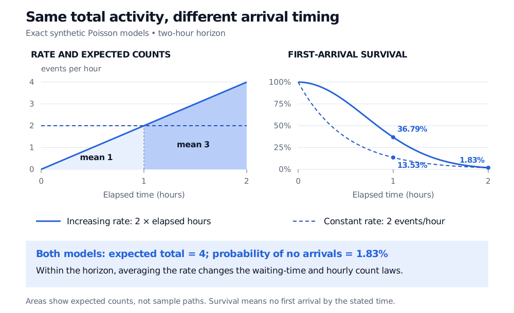
The instantaneous rate starts at zero and reaches 4 events per hour. The integrated intensity is $\Lambda(t)=(t/\text{hour})^2$ in event-count units. The area under the rate curve gives:

Window	Count mean	Probability of no requests
First hour	1	$e^{-1}\approx36.79\%$
Second hour	3	$e^{-3}\approx4.98\%$
Full two hours	4	$e^{-4}\approx1.83\%$

The second-hour count is independent of the first-hour count, although its distribution is different. The process lacks stationary increments: equal durations need not have the same count law.

Replacing the curve with its two-hour average, 2 events per hour, preserves the full-period Poisson count law. It gives each hour mean 2, however, and therefore misses the timing of the workload. A capacity decision tied to the busiest hour needs more than the full-period total.

A rate increasing linearly from zero to four events per hour has first-hour area one and second-hour area three. Its first-arrival survival is 36.79 percent at one hour and 1.83 percent at two hours. A constant two-per-hour comparison has one-hour survival 13.53 percent and the same two-hour survival.

Original exact synthetic model. Shaded areas are expected counts, not realised arrivals. Both rate profiles give total mean four; their first-arrival survival curves differ within the horizon.

Waiting uses the accumulated rate too

Let $T_1$ be the first arrival time. No first arrival by $t$ means no events by $t$ , so

\mathbb{P}(T_1>t)=e^{-\Lambda(t)}.

In the example this is

e^{-(t/\text{hour})^2}

for

0\le t\le2\,\text{hours}

, rather than constant-rate exponential survival. The rate is zero at the initial instant, yet the probability of an arrival during the first hour is positive: an instantaneous rate is not a whole-window probability.

More generally, starting at a fixed clock time $s$ , the probability of waiting at least a further $u$ is

\mathbb{P}(N_{s+u}-N_s=0) =\exp\bigl(-[\Lambda(s+u)-\Lambda(s)]\bigr).

This depends on the starting time. Successive gaps between arrivals are generally neither independent nor identically distributed in calendar time; independent counts in fixed disjoint windows do not imply independent gaps whose endpoints are random arrival times. A model specified only through two hours also leaves later waits unspecified: paths with no arrival by the horizon are censored there.

A different clock, and a modelling boundary

One construction is

N_t=M_{\Lambda(t)}

, where

M

is a unit-rate Poisson process. Independent exponential gaps then live in integrated-intensity time. Converting back to hours changes their spacing. This deterministic time change works even when the rate vanishes on an interval; the count simply stays constant there. See Gallager's MIT notes, §2.4 for the construction.

For a fuller foundation, Defining the Poisson Process: Three Equivalent Constructions connects the constant-rate construction to the nonhomogeneous count law; the preview is public and full reading requires membership.

A changing deterministic rate explains predictable seasonality. It does not establish that arrivals in real order flow are independent, nor capture arrivals that trigger further arrivals. Random or history-dependent intensity belongs to a broader point-process model. Rate seasonality and event-driven clustering answer different questions.

Sources

Richard Durrett, Essentials of Stochastic Processes, third edition, Springer, 2016, §2.2, “Nonhomogeneous Poisson Processes,” pp. 105–106; §2.4.1, Theorem 2.12.
Robert G. Gallager, Discrete Stochastic Processes, Chapter 2, §2.4, MIT OpenCourseWare — integrated-rate counts and deterministic time change.

The rate is a curve; its area is the expected count

Two equal hours, unequal activity

Waiting uses the accumulated rate too

A different clock, and a modelling boundary

Sources

Related terms

Exponential distribution

Independent increments

Intensity of a point process

Poisson distribution

Poisson process

Stationary increments