A conditional arrival rate uses the event history. Distinguish instantaneous intensity, its accumulated compensator and an average rate, with a rising-rate Poisson example.
Intensity of a point process
The intensity of a point process is a rate describing how quickly events are expected to arrive. For a temporal process, conditional intensity means the rate given the information available just before the current time. An execution model can use it to distinguish predictable intraday activity from arrivals that become more likely after earlier orders. A historical total divided by elapsed time does not make that distinction.
Let Nt be a simple counting process: it starts at zero and jumps by one at each event, with finitely many arrivals in every bounded interval. Let the filtrationFt specify the information observed by time t. The conditional intensity λt has units of events per unit time. Informally,
E[dNt∣Ft−]=λtdt.
This is infinitesimal shorthand, rather than an equality for an arbitrary finite window. Under the usual local regularity and negligible-multiple-arrival conditions, λth is also a first-order approximation to the conditional probability of an arrival in a sufficiently short interval of length h. The rate itself can exceed one; a probability cannot.
The history in the conditioning matters. In spatial point-process work, “intensity” often means an unconditional mean density of points. For a temporal model with an integrable conditional intensity, the mean rate is E[λt] almost everywhere. That average generally differs from the current, history-dependent λt. Rasmussen's lecture notes introduce this conditional view through the distribution of the next event.
The accumulated rate is the compensator
The precise definition uses a predictable process: the rate must use information available before the event it predicts. Suppose the count has finite expectation on each finite horizon and its compensator is absolutely continuous in time. Then an intensity is a nonnegative predictable process satisfying
At=∫0tλsds,Mt=Nt−At,
where Mt is a martingale relative to the chosen filtration. The compensator At accumulates the rate; subtracting it removes the count's predictable drift. Slud's counting-process notes develop this decomposition.
With these integrability assumptions, its useful forecasting implication is
E[Nv−Nu∣Fu]=E[∫uvλsdsFu],0≤u<v.
If future intensity is random, the integral on the right is random too: it still needs a conditional expectation. Neither the realised accumulated intensity At nor today's rate alone is generally a forecast for the entire future window. The information set is part of the model; changing what is observed can change the conditional intensity.
Not every point process has an intensity with respect to ordinary time. A certain event scheduled at a known instant produces a jump in its compensator, which cannot be represented by a finite rate integrated against dt. The absolute-continuity assumption excludes such predictable atoms; see Björk’s treatment of intensity existence and filtration, §§3.2–3.5.
One rising rate, three different numbers
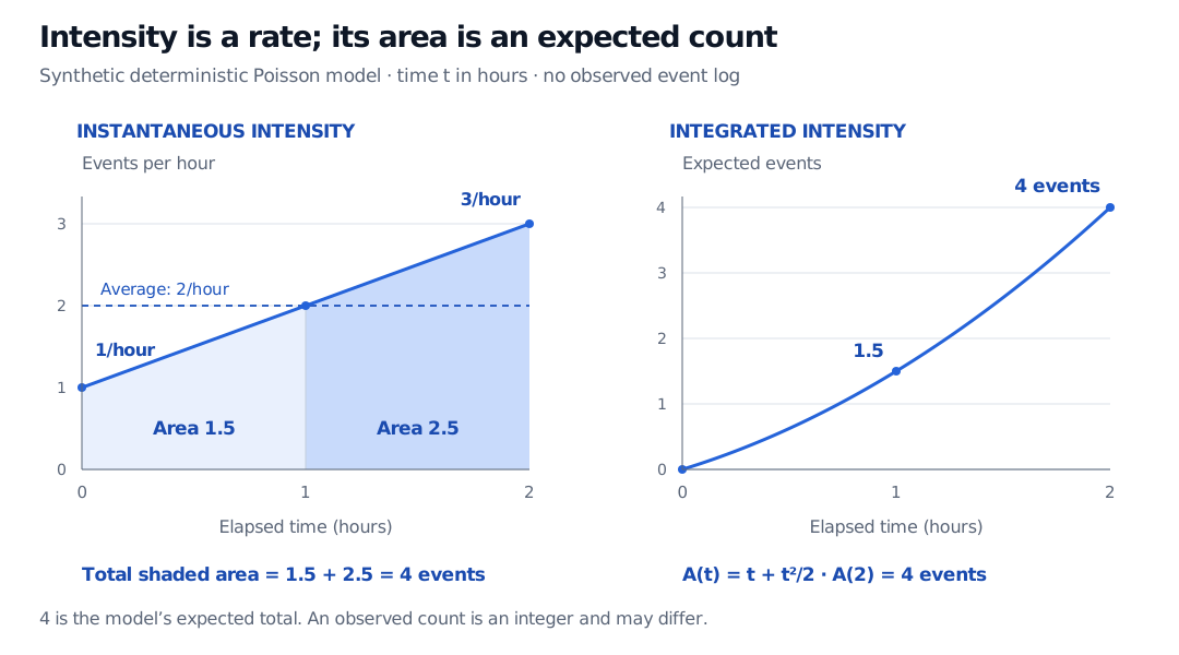
Consider a synthetic request-arrival model over two hours, starting with no requests counted. Assume a nonhomogeneous Poisson process whose deterministic intensity is
λ(t)=hour1+hour2t,0≤t≤2hours.
The rate rises from 1 event per hour to 3 events per hour. Because it is deterministic, there is no uncertainty about the future rate curve in this example. The integrated intensity is the area under it:
A2hours=∫02hoursλ(s)ds=4.
Quantity
Value
What it describes
Endpoint intensity
3 events/hour
Local rate at the end of the window
Average intensity over the window
2 events/hour
Integrated intensity divided by two hours
Integrated intensity
4 events
Expected count across the full window
Multiplying the endpoint rate by two hours would give 6 events, overestimating the model's expected count. That calculation incorrectly treats the final rate as if it had applied throughout the period. The actual area is 1.5 expected events in the first hour plus 2.5 in the second.
Synthetic deterministic intensity rises from 1 to 3 events per hour over two hours. Its average is 2 per hour, and its area is 4 expected events, split into 1.5 and 2.5 across the two hours. The integrated-intensity curve reaches 4 at two hours.
Original deterministic Poisson example. Left: the rate and its shaded area. Right: accumulated intensity, measured in expected events. Neither curve is an observed count path.
The Poisson assumption, together with this deterministic rate, gives
N2hours∼Poisson(4),P(N2hours=0)=e−4≈1.83%.
An expected count of four does not guarantee four arrivals. A zero-length window has integrated intensity zero and count zero; an identically zero rate gives no arrivals. Units remain essential: an hourly rate must be integrated over hours, or converted consistently before using minutes.
For the deterministic Poisson special case, Defining the Poisson Process: Three Equivalent Constructions extends the constant-rate definition to integrated time-varying rates. The public page is a preview; the full lesson requires membership.
A stochastic rate does not automatically give Poisson counts
A constant deterministic conditional intensity gives the usual homogeneous Poisson process. A deterministic time-varying intensity gives the nonhomogeneous version. By contrast, a Hawkes process lets earlier events increase later intensity. Its current rate describes local activity; it does not make the next hour's count Poisson with mean “current rate times one hour.” Future events can change that rate again.
A Cox process has a different construction: conditional on its full random directing-intensity path, it is Poisson. Conditioning only on today's intensity value is less information and does not generally produce that count law. Under a smaller observed-information filtration, even the conditional intensity is a filtered rate rather than necessarily the unobserved directing rate itself.
For a single possible default, the closely related hazard rate is conditional on survival. The default-count intensity includes the indicator that default has not yet occurred; after default, that one-name count cannot jump again. Intensity specifies arrival timing, while the loss at default needs its own model.
Sources
Richard Durrett, Essentials of Stochastic Processes, third edition, Springer, 2016, §2.2.2, pp. 105–106: deterministic nonhomogeneous Poisson intensity, integrated count law and first-arrival survival.