A counting process is a stochastic process that records how many events have occurred by each time. In an execution study, it might count incoming orders; in credit risk, defaults. It describes event timing and totals, while order size, execution price and loss severity require additional variables.
Using the convention here, and counts events in . Paths are nonnegative, integer-valued, nondecreasing and right-continuous, with finitely many events on every bounded time interval. Right-continuity means an event at time is already included in .
Some authors reserve “counting process” for simple processes, whose jumps all have size one. Here the broader convention allows a jump larger than one when several events occur together; a simple counting process excludes such coincidences. State the convention before interpreting a jump.
One event log, several useful readings
Suppose a synthetic order log contains four arrivals at 0.5, 1.5, 2 and 3 hours after the observation origin. These are stipulated times, not simulated Poisson arrivals. For positive event times , the count is
where each indicator contributes one once its event has arrived. Before observing the log, random event times define a process; this particular log determines one realised path.
| Time after origin (hours) | Count |
|---|---|
| 0 | 0 |
| 0.5 | 1 |
| 1 | 1 |
| 2 | 3 |
| 3 | 4 |
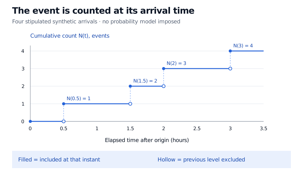
Original diagram of the stipulated event log. Filled dots include each arrival at its exact time; hollow dots show the excluded previous level. No arrival law is assumed.
The count in a later window is an increment:
For , this is event. The arrival at 1.5 hours is excluded; the arrival at 2 hours is included. This convention lets adjacent windows partition the log without counting a boundary event twice.
The same log also gives waiting times: 0.5 hours from the origin to the first arrival, followed by gaps of 1, 0.5 and 1 hour. Waiting times have time units; counts have event units. The observed average over the first three hours is events per hour. That ratio is a descriptive rate, not by itself a conditional intensity or a forecast for the next hour.
The staircase does not choose the arrival model
A counting process need not be a Poisson process. Its definition supplies neither a constant intensity nor independent increments. A model can allow seasonality, dependence on earlier arrivals, or other timing patterns while retaining the counting structure. Observing four events alone does not determine probabilities for future totals or waiting times.
Nor does an integer-valued state make the clock discrete: is defined for every real . Recording it only at hourly checkpoints gives a sampled discrete-time process, which can hide events occurring between observations. Timestamp rounding can also make distinct events appear simultaneous; distinguish that recording limitation from actual simultaneous arrivals.
For a specific probabilistic model built on this bookkeeping, Defining the Poisson Process: Three Equivalent Constructions connects counts with exponential waiting times. Its public page provides a preview; the full lesson requires membership.
Sources
- Miltiadis C. Mavrakakis and Jeremy Penzer, Probability and Statistical Inference: From Basic Principles to Advanced Models, first edition, CRC Press, 2021, §6.7, pp. 198–199: counting paths, right-continuity and interval increments.
- Hao Wu, MIT OpenCourseWare, 18.445, Lecture 20, 29 April 2015, slides 2–3: arrival times, non-explosion and counts on .
- Tomas Björk, Point Processes and Jump Diffusions, Chapter 1 publisher excerpt, Definition 1.1: the stricter unit-jump convention, contrasted here with the broader counting convention.