Standard Brownian motion has zero drift and unit variance rate. See how time units, independent shocks, dependent levels and conditional forecasts fit together.
Standard Brownian motion
Standard Brownian motion is a continuous random process that starts at zero and has independent Gaussian increments with mean zero and variance equal to elapsed time. “Standard” fixes the drift at zero and the variance rate at one. That normalization lets a financial model specify the size of its random shocks through a separate volatility coefficient.
For a standard Brownian motion written (Wt)t≥0, the complete definition requires:
W0=0 almost surely.
For 0≤s<t, Wt−Ws∼N(0,t−s), where the second parameter is variance.
Increments on disjoint time intervals are independent.
With probability one, the entire path t↦Wt is continuous.
The normal distribution of an increment depends only on its interval's length: a quarter-year shock has the same distribution whether it occurs in the first or the fifth year. This is stationarity of increments. The levels themselves are not stationary, because their variance grows with time. See Lalley's definition of the Wiener process, §1.1.
Standard does not mean unit variance at every date
Setting s=0 gives
E[Wt]=0,Var(Wt)=t,SD(Wt)=t.
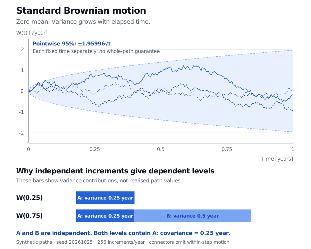
If time is measured in years, Wt carries square-root-year units. Its standard deviation is 0.5year at t=0.25 year and 1year at t=1 year. Four independent quarter-year increments add their variances to one year; their standard deviations do not add.
At each fixedt>0, the central 95% normal interval is approximately
[−1.95996t,1.95996t].
Its endpoints are approximately ±0.980year at a quarter year and ±1.960year at one year. This is a pointwise distributional statement. It does not give a 95% probability that a whole path stays inside the displayed envelope.
Three synthetic standard Brownian paths with pointwise 95% normal intervals; quarter-year SD is 0.5 square-root year and one-year SD is 1. Below, shared variance 0.25 year explains dependence between W at 0.25 and 0.75 year.
Original model illustration: three seeded Gaussian-grid paths, seed 20261025, 256 intervals over one year. Dashed bounds show pointwise central 95% intervals. Bars below show variance contributions, not realised values; straight path connectors omit within-step motion.
New shocks are independent; accumulated levels share history
Let A=W0.25 and B=W0.75−W0.25. Then
A∼N(0,0.25),B∼N(0,0.50),A and B are independent.
Here and below the time coordinate is numerical years, so the variances have year units. Although B is fresh noise, W0.75=A+B still contains the earlier level A. Consequently,
Cov(W0.25,W0.75)=Cov(A,A+B)=Var(A)=0.25 year.
Their correlation is 0.25/0.25×0.75=1/3≈0.5774. More generally,
Cov(Ws,Wt)=min(s,t).
Zero drift means the conditional mean forecast of a future level is today's level, rather than zero. With the process's natural filtrationFs, which records its history through s,
Wt∣Fs∼N(Ws,t−s),t>s.
The first and third faces in the membership lesson The Four Faces of Brownian Motion develop the conditional-mean and covariance calculations. The link offers a public preview; the full lesson requires membership.
Sampling the driver, then choosing a financial model
On a specified grid 0=t0<t1<⋯<tn, draw independent Zi∼N(0,1) and set
Wti=Wti−1+ti−ti−1Zi.
This samples the exact joint law at the grid points. Connecting the points does not reveal the intervening Brownian path or determine whether it crossed a barrier. A finite plot cannot establish an almost-sure path property.
In a financial model, σWt scales the noise. For example, a return model with σ expressed per square-root year has a dimensionless return shock σ(Wt−Ws). Changing the time unit requires changing the coefficient consistently. Lawler, §§2.4 and 2.6, develops the standard normalization and Brownian scaling.
Wt can take negative values. To model a positive asset price, one possible choice is geometric Brownian motion, which transforms this driver through an exponential. Independent Gaussian shocks and continuous paths are assumptions of that model, not conclusions about how markets must behave.
Practice: what changes after an observation?
Time is in years. You observe W0.16=0.30year. What are the conditional mean and variance of W0.64?
Answer. The new increment is independent of the observed history and has mean zero and variance (0.64−0.16)=0.48 year. Adding it to the observed level gives conditional mean 0.30year, variance 0.48 year and standard deviation 0.48≈0.692820year. The unconditional mean zero and variance 0.64 year describe the level before incorporating the observation; they are not the updated forecast.
Sources
Gregory F. Lawler, Stochastic Calculus: An Introduction with Applications, revision of 15 February 2023, §§2.4 and 2.6: author's University of Chicago text.