Compound Poisson process: Definition & Examples

A compound Poisson process adds a random amount at each arrival of a Poisson process. The Poisson process supplies the event times; independent, identically distributed marks supply the amounts. For aggregate losses, this separates how often loss events occur from how large each loss is. Counting claims alone cannot measure the uncertainty in their total cost.

Write the accumulated amount as

C_t=\sum_{i=1}^{N_t}J_i,\qquad C_0=0,

where $N_t$ is a homogeneous Poisson process of rate $\lambda$ , the marks $J_i$ are i.i.d., and the entire mark sequence is independent of the arrival process. An empty sum is zero. The time parameter is continuous, while a path is constant between arrivals and changes by the next mark when an event occurs. Marks may be positive, negative or zero; a loss-only interpretation usually uses nonnegative marks.

Six expected events is still a random number

Consider a synthetic event-cost model, with no claim of calibration to actual losses. Events arrive at rate 2 per hour. Each independently costs USD 1 with probability 75%, or USD 3 with probability 25%. Over three hours, the expected count is

\lambda t=6

. It does not follow that six events will occur.

The mark moments are

\begin{aligned} \mathbb{E}[J]&=0.75(1)+0.25(3)=1.5\ \text{USD},\\ \mathbb{E}[J^2]&=0.75(1^2)+0.25(3^2)=3\ \text{USD}^2,\\ \text{Var}(J)&=3-1.5^2=0.75\ \text{USD}^2. \end{aligned}

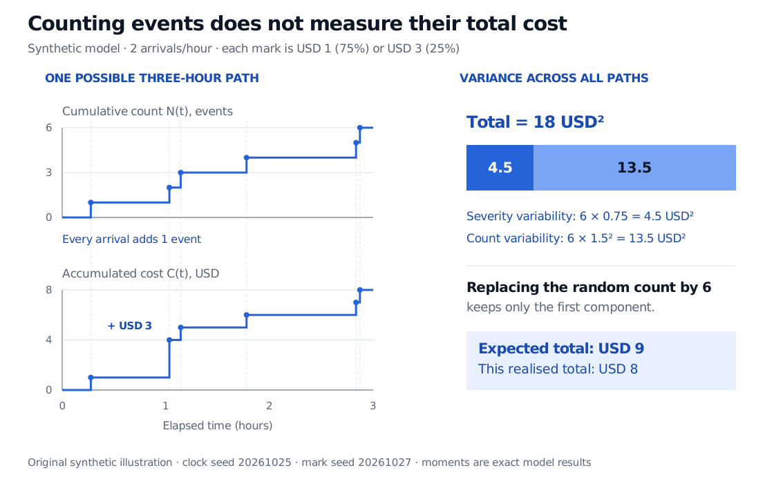
Consequently, the expected three-hour cost is USD 9, while its variance is 18 USD². A particular realisation can be much smaller or larger. The original seeded path below happens to contain six events whose costs sum to USD 8.

Synthetic three-hour path has six events and accumulated cost USD 8. At the same arrivals, the count jumps by one while costs jump by USD 1 or USD 3. Exact aggregate variance 18 USD squared comprises severity variability 4.5 and count variability 13.5.

Original synthetic illustration; clock seed 20261025 and mark seed 20261027. Both paths use the same arrivals. The variance decomposition describes the model across all paths, rather than the variability within this single path.

Why the second moment appears

The law of total variance exposes what would be lost by replacing the random count with its mean. Conditional on $N_t=n$ , the total is a sum of exactly $n$ independent marks:

\mathbb{E}[C_t\mid N_t=n]=n\mathbb{E}[J],\qquad \text{Var}(C_t\mid N_t=n)=n\text{Var}(J).

Averaging over the count gives, when the relevant moments are finite,

\begin{aligned} \mathbb{E}[C_t]&=\lambda t\,\mathbb{E}[J],\\ \text{Var}(C_t) &=\mathbb{E}[N_t]\text{Var}(J) +\text{Var}(N_t)\big(\mathbb{E}[J]\big)^2\\ &=\lambda t\,\mathbb{E}[J^2]. \end{aligned}

In the cost example, the two contributions are

6(0.75)=4.5

USD² from severity variability and

6(1.5^2)=13.5

USD² from count variability. Their sum is 18 USD². Using

6\text{Var}(J)=4.5

USD² alone would describe the variance of a sum with a fixed count of six. It omits the uncertainty about how many costs are incurred.

A useful limiting check is to make every mark the same nonzero amount $c$ . The marks then have zero variance, but $C_t=cN_t$ remains random: its variance is $c^2\lambda t$ . Count uncertainty survives even when severity uncertainty disappears.

For a longer derivation and the connection to splitting arrivals into independent mark classes, see Superposition, Thinning, and Compound Poisson Processes. The full lesson requires membership; its preview is public.

Zero total does not always mean zero events

In this example every mark is strictly positive. Therefore the total is zero exactly when no event occurs:

\mathbb{P}(C_3=0)=\mathbb{P}(N_3=0)=e^{-6}\approx0.25\%.

That equivalence needs the positivity assumption. With nonnegative marks that may equal zero, events can occur without increasing the total. If $p_0=\mathbb{P}(J=0)$ , independent Poisson thinning gives $\mathbb{P}(C_t=0)=\exp[-\lambda t(1-p_0)]$ . With signed marks, positive and negative jumps may cancel as well; neither shortcut applies in general.

What carries over, and what does not

A compound Poisson process has stationary, independent increments: totals over disjoint time intervals are independent, and the law of an increment depends on the interval's length. These properties follow from the arrival assumptions and the independent marks. Over a finite interval there are finitely many arrivals almost surely, so this is a finite-activity jump process.

Those are strong modelling commitments. A common stress event can make losses arrive together or make later losses larger; mark distributions can also change with time. Such behaviour is not supplied by a homogeneous compound Poisson specification. Adding signed marks also does not, by itself, produce a complete asset-price model: discounting, drift and the pricing measure still need their own assumptions.

Sources

Richard Durrett, Essentials of Stochastic Processes, third edition (2016), §2.3, pp. 106–108, especially Theorem 2.10: random-sum moments and their interpretation.
Kyle Siegrist, Compound Poisson Processes, Random: Probability, Mathematical Statistics, Stochastic Processes: independent marks, stationary independent increments, moments and the discrete thinning construction.

Six expected events is still a random number

Why the second moment appears

Zero total does not always mean zero events

What carries over, and what does not

Sources

Related terms

Poisson process