Volatility skew is the asymmetry of implied volatility across strikes for options on the same underlying, observed at the same time and with the same expiry. A downward skew means lower strikes have higher implied volatilities than higher strikes. It is common in equity-index options, where downside protection can carry a substantial volatility premium. OIC defines skew through this same-expiry comparison.
The comparison concerns a price quotation: implied volatility is the volatility input that makes a chosen option-pricing model reproduce an option price. It is not a separate forecast attached to each possible future stock price. In the constant-volatility Black–Scholes model, the fixed-expiry curve would be flat. Market prices need not fit that restriction.
A floor costs more than the flat-volatility benchmark
A portfolio manager wants six-month protection below USD 80 on an underlying currently worth USD 100. Consider these hypothetical European option quotes, all for that six-month expiry. Set interest rates and dividend yield to zero, so the corresponding forward is also USD 100. Volatilities are annualised Black–Scholes implied volatilities.
| Strike , USD | Strike / forward | Implied volatility | Difference from the 100-strike IV |
|---|---|---|---|
| 80 | 0.8 | 35% | +10 percentage points |
| 100 | 1.0 | 25% | 0 |
| 120 | 1.2 | 22% | −3 percentage points |
The 80-strike put buys protection against a large fall. Its 35% IV is 10 volatility percentage points above the at-the-money quote. That is a 40% relative increase from 25%, rather than a 10% relative increase. The upside 120-strike call has an IV three percentage points below the middle quote. The whole pattern slopes downward, with a much larger departure on the downside.
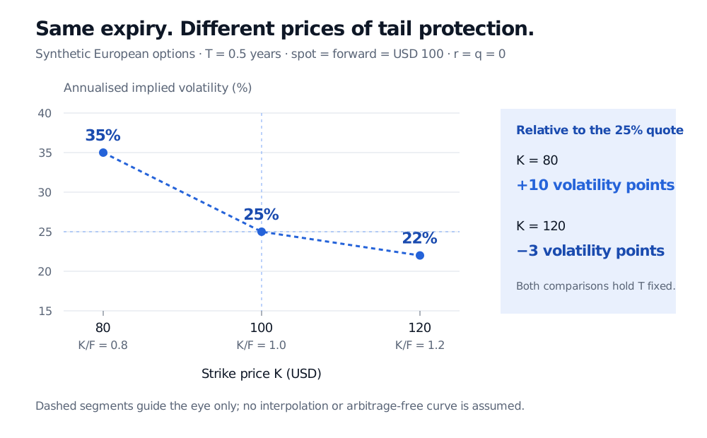
Original synthetic quotes; six-month European options, zero interest rate and dividend yield. Dashed segments guide the eye between the three points; they do not assert an arbitrage-free interpolation.
What does the extra volatility mean in money? For the same 80-strike put, Black–Scholes gives a premium of approximately USD 2.21 per underlying unit at 35% IV, compared with USD 0.78 at a flat 25% IV. The difference is about USD 1.43. Both calculations use spot 100, half a year to expiry and zero carry. This is a comparison of two valuations of the same contract, not a claim that the manager can buy at the lower price.
Calling the put wing “rich” describes its higher IV relative to a benchmark. It does not establish that selling protection earns an attractive return: the seller takes the loss exposure that the buyer wants to transfer. Nor does a higher IV mean a larger dollar premium than every lower-IV option. Strike, expiry and the rest of the contract still affect the price.
The slope needs an axis and a sign convention
A volatility smile is the broader non-flat relationship between IV and strike; skew describes its asymmetry or slope. A curve can have both curvature and skew. For a fixed expiry , write its IV as .
Raw strikes make comparisons across underlyings awkward: a ten-dollar strike gap means something different for an asset worth 20 than for one worth 2,000. Moneyness supplies a relative axis. Common choices are and log-forward-moneyness
Here is the forward price for the option's expiry. At-the-money-forward means ; it need not mean strike equals today's spot when carry is nonzero. A local ATM skew is often defined as
A downward-sloping curve has a negative slope under either increasing-strike axis. But a low-strike IV minus high-strike IV spread is positive for the same curve: the example gives volatility percentage points. State which quantity you mean. Three discrete quotes do not uniquely determine an ATM derivative without an interpolation assumption, and an IV slope is not a dollar vega.
“Put skew” also does not mean that a put must have a higher IV than a call at the same strike. Matched European calls and puts satisfying put–call parity have the same Black–Scholes IV when inverted using consistent carry and contract inputs. The usual wing comparison uses low-strike out-of-the-money puts and high-strike out-of-the-money calls. The example's equally spaced strikes are not equally spaced in log-moneyness or necessarily matched in absolute delta.
What the shape tells you—and what it cannot
Demand for crash protection, the compensation required to bear downside risk, jumps and the tendency for equity volatility to rise in falling markets can all contribute to downward skew. Hull discusses leverage and crash concerns as explanations. The shape alone cannot identify a unique cause or tell you that a particular trade is mispriced.
Keep three different questions separate:
| Object | What changes in the comparison? | What it describes |
|---|---|---|
| Fixed-expiry volatility skew | Strike or moneyness; expiry stays fixed | Relative option prices expressed as IV |
| Volatility term structure | Expiry; the chosen moneyness convention stays fixed | How annualised IV varies across horizons |
| Skewness of realised returns | Observations in a return sample | A distribution's asymmetry, measured through a standardised third central moment |
A full volatility surface combines the strike and expiry dimensions. One expiry can have a steep downside skew while its ATM term structure slopes upward, downward or remains flat.
Option prices reflect risk-neutral pricing, including compensation for bearing risk, rather than unadjusted real-world outcome probabilities. A downward IV skew is therefore not a numerical forecast of a crash probability or the measured skewness of past returns. Even recovering a risk-neutral terminal distribution requires a suitably regular, arbitrage-consistent range of option prices—not just the three quotes above. A snapshot also does not specify how the skew will move when spot changes.
For a visual experiment, open the public Volatility Surface explorer, select Downside skew, hold the expiry selection fixed and compare strikes. Then change Skew and Term slope separately. The explorer uses a synthetic parametric surface with a constant forward across expiries; it is not live market data, a fit to this example or a guarantee of no arbitrage. With actual quotes, check timestamps, bids and asks, exercise style, carry and settlement conventions before interpreting a wing difference. Small price errors can produce large IV errors when vega is small.
Sources
- John C. Hull, Options, Futures, and Other Derivatives, 9th Global Edition, §§20.1 and 20.3–20.5: matched European call/put IVs, equity skew, moneyness conventions, term structure and surfaces. All quotes, calculations and the figure here are original hypothetical examples.
- Options Industry Council: April Webinar Key Takeaways—Understanding Volatility and Options Skew, April 2026: same-expiry strike comparisons, asymmetric wing demand and the distinction from term structure.