Volatility regime adjustment: Definition & Examples

Volatility regime adjustment rescales a risk model's volatility forecasts using recent evidence that realised shocks are collectively larger or smaller than their predicted scale. In a factor risk model, a common multiplier can raise the entire factor-risk forecast quickly while preserving its correlation structure. This affects the risk assigned to a portfolio before the slower underlying estimates have fully adapted.

The historical MSCI USE4 methodology, §4.3, describes a multiplier estimated from cross-sectional factor returns standardised by their start-of-day forecasts. The construction below follows that August 2011 framework; its illustrative weights are stipulated, not current vendor calibration parameters.

Build the signal from forecasts recorded beforehand

Let $f_{k,s}$ be factor $k$ 's realised return on completed day $s$ , and $\widehat\sigma_{k,s}>0$ its one-day volatility forecast recorded at that day's start. With $K$ factors, define

z_{k,s}=\frac{f_{k,s}}{\widehat\sigma_{k,s}}, \qquad q_s=\frac1K\sum_{k=1}^{K}z_{k,s}^2.

For normalised nonnegative lookback weights $a_{t,s}$ , define the multiplier available after day $t$ as

\lambda_t^2=\sum_{s\le t}a_{t,s}q_s, \qquad \sum_{s\le t}a_{t,s}=1.

The historical method uses exponential time weights. Here

\lambda_t

can adjust a subsequent forecast: day

t

's realised return cannot inform its own start-of-day prediction. This timing is essential to backtesting.

The cross-sectional quantity

\sqrt{q_s}

is an uncentred RMS, with division by

K

. It differs from the temporal sample standard deviation used for the risk-model bias statistic in Appendix A. Squaring, weighting and taking a square root do not commute.

This raw-return construction treats expected daily factor returns as negligible. If conditional means matter, $q_s$ also picks up their squared contribution; it is not a pure variance diagnostic.

Two observations, one common scale

Take two fictional factors and only two completed daily observations. Their standardised shocks and declared weights are:

Observation	Factor 1	Factor 2	Mean square $q_s$	Time weight
Previous	0	0	0	0.25
Latest	2	0	2	0.75

Thus

\lambda_t^2=0.25(0)+0.75(2)=1.5, \qquad \lambda_t=\sqrt{1.5}\approx1.224745.

Averaging the daily RMS values instead would give $0.25(0)+0.75\sqrt2\approx1.060660$ . That is a different statistic and the wrong multiplier for this definition. The example is an arithmetic illustration, not evidence that two dates suffice to calibrate a model.

Suppose the base one-day factor covariance forecast is

F=\begin{pmatrix}0.04&0.01\\0.01&0.09\end{pmatrix}.

Returns here are measured in percentage points, so the entries are in percentage points squared. Applying the adjustment gives

\widetilde F=\lambda_t^2F =\begin{pmatrix}0.06&0.015\\0.015&0.135\end{pmatrix}.

Factor volatilities rise from $0.2$ and $0.3$ percentage points to approximately $0.244949$ and $0.367423$ percentage points. Covariances rise by 50%; volatilities rise by approximately 22.47%. Multiplying $F$ by $1.224745$ would apply a volatility ratio directly to squared units.

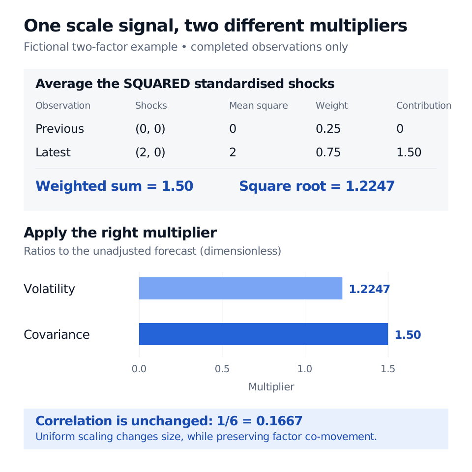
Fictional two-factor example: previous standardised shocks (0, 0) and latest (2, 0) have mean squares 0 and 2. Weights 0.25 and 0.75 give covariance multiplier 1.50 and volatility multiplier 1.2247. Factor correlation stays 1/6, approximately 0.1667.

Original stipulated example. Average the squared standardised shocks before taking a square root; the two multipliers act on different risk quantities.

For these two factors, correlation is unchanged:

\rho=\frac{0.01}{\sqrt{0.04(0.09)}}=\frac16, \qquad \widetilde\rho=\frac{0.015}{\sqrt{0.06(0.135)}}=\frac16.

More generally, the common positive variance multiplier cancels from every factor correlation. For any fixed factor-exposure vector $\mathbf x$ , $\mathbf x^\top\widetilde F\mathbf x=\lambda_t^2\mathbf x^\top F\mathbf x$ . Every such direction receives the same proportional variance adjustment. Its relative risk ranking is preserved.

A scale correction has a limited job

The common adjustment cannot repair a mistaken factor correlation or a missing risk driver. In contrast, eigenfactor risk adjustment targets selected covariance directions rather than a single common scale. Nor does a large recent

q_s

prove a lasting regime change: one extreme shock can dominate the signal, and correlated factors do not provide independent observations. A shorter lookback reacts faster and also makes the scale estimate more sensitive to recent noise.

Factor and idiosyncratic risk need not receive the same multiplier. USE4 §5.3 estimates a separate specific-risk adjustment. With exposure matrix

B

, base specific covariance

D

, and separately estimated positive multipliers, the model becomes

\widetilde\Sigma =B(\lambda_F^2F)B^\top+\lambda_S^2D.

Consequently, unchanged factor correlations do not establish unchanged asset correlations when

\lambda_F\ne\lambda_S

. Total portfolio volatility also need not rise by

\lambda_F

when specific risk is present.

Risk Models: APT and Factor Structure derives this factor-plus-specific covariance decomposition. Its public page provides a preview; the full lesson requires membership. For the broader forecasting problem, see volatility forecasting. A historical adjustment rule alone does not establish future forecast accuracy or describe today's vendor products.

Sources

Menchero, J., Orr, D. J. and Wang, J. (August 2011), The Barra US Equity Model (USE4): Methodology Notes, §4.3, pp. 24–27, equations 4.3–4.5; §5.3, pp. 31–34, equations 5.10–5.12; Appendix A, pp. 36–39. Historical MSCI-authored methodology hosted by a third-party mirror.

Build the signal from forecasts recorded beforehand

Two observations, one common scale

A scale correction has a limited job

Sources

Related terms

Backtesting

Correlation

Covariance

Eigenfactor risk adjustment

Idiosyncratic risk

Risk-model bias statistic

Volatility forecasting