How eigenfactor risk adjustment calibrates selected covariance directions, why volatility multipliers are squared, and why corrected variances do not recover the true covariance.
Eigenfactor risk adjustment
Eigenfactor risk adjustment recalibrates the variances assigned to the eigenvector directions of an estimated factor covariance matrix to reduce risk forecast bias caused by sampling error. Its practical target is a portfolio optimiser's tendency to concentrate in directions whose estimated risk is unusually low. It changes the risk matrix used for construction, rather than adding one blanket buffer to the final portfolio volatility.
Menchero, Wang and Orr develop this approach in Improving Risk Forecasts for Optimized Portfolios. Their eigenportfolios reveal strong underprediction in low estimated variance directions and some overprediction at the high end. These are empirical findings under their research design, not universal multipliers.
Why an unbiased matrix can mislead an optimiser
For a covariance estimate F satisfying E[F]=F, a fixed, nonrandom exposure vector a has
E[a⊤Fa]=a⊤Fa.
That equality does not establish unbiased risk forecasts for a direction u selected using the same estimated matrix. The direction and estimation errors then depend on each other. Selecting the smallest estimated variance preferentially finds errors that make risk look cheap. Unbiased variance estimation also does not imply unbiased volatility estimation, because taking a square root is nonlinear.
The columns uk are unit-length factor exposure directions. Their estimated variances are dk, and they are mutually uncorrelated under this estimated matrix. The smallest eigenvector minimises u⊤Fu subject to u⊤u=1. This is a unit-norm problem; a budget constraint such as weights summing to one defines a different portfolio problem. The authors' May 2011 research paper, “Eigenfactors”, explains this distinction.
Use the observed covariance as the generating covariance inside the simulation.
Generate synthetic factor histories; refit the same covariance estimator.
Diagonalise each refit; compare each eigenportfolio's forecast variance with its variance under the generating covariance.
Aggregate comparisons by eigenfactor rank into volatility correction factors vk.
The reconstruction is
Fadj=Udiag(v12d1,…,vK2dK)U⊤.
A volatility multiplier must be squared when applied to a variance. The original eigenvectors are retained. Known simulation truth is not knowledge of the real population covariance.
Two corrected directions still leave a missing covariance
Consider a stipulated oracle illustration, with all entries in common squared-return units at one fixed horizon:
The estimated eigenvectors are the coordinate axes, so U=I. Supply the true matrix only to demonstrate the arithmetic; no return sample or Monte Carlo fit produces these numbers.
Both coordinate directions have true variance 0.025. Their variance ratios and volatility multipliers are therefore
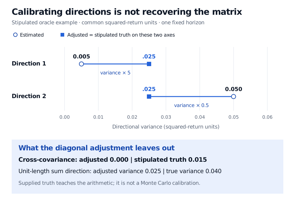
The first direction's variance rises fivefold; the second's halves. Applying vk2=rk gives
Fadj=(0.025000.025).
Stipulated oracle example. Direction 1 variance moves from 0.005 to 0.025 and direction 2 from 0.050 to 0.025. Adjusted cross-covariance remains zero although stipulated truth is 0.015. Along the unit-length sum direction, adjusted variance is 0.025 versus true variance 0.040.
Original stipulated oracle example: the two directional variances match, while the cross-covariance remains missing. These are supplied calibration ratios, not estimates from a vendor simulation.
This adjustment does not recover Ftrue. Its off-diagonal entry stays zero. For the unit-length combined direction a=(1,1)⊤/2,
Matching the two chosen directional variances does not match every combination. The true matrix has eigenvalues 0.010 and 0.040; they are not the two 0.025 directional variances measured along the estimated axes. The axes themselves differ from the true eigendirections. The trace also changes, from 0.055 to 0.050: trace preservation is not imposed here.
Read the calibration in context
This is distinct from covariance eigenvalue clipping, which can pool a designated noise group at one average, and from fitted nonlinear covariance shrinkage. Equal adjusted eigenvalues in this example are a consequence of the supplied ratios, not a clipping rule.
The USE4 document assumes normal, stationary simulated returns and discusses the limits of that approximation. It also distinguishes an additional empirically scaled correction from the milder simulated correction adopted in that historical model. These August 2011 choices are not a specification or performance guarantee for today's products. Appendix B, equations B7–B10, gives the details.
A correction trained on one estimated covariance and sampling scheme cannot establish that every future portfolio forecast is calibrated. Constraints, changing covariance and factor-model omissions still matter. Evaluate risk forecasts on portfolios formed with information available at the time.
For the portfolio construction step, Mean–Variance Optimisation derives inverse-covariance weights and the fully invested constraint. Its public page is a preview; the full lesson requires membership.
Sources
Menchero, J., Wang, J. and Orr, D. J. (2012), Improving Risk Forecasts for Optimized Portfolios, Financial Analysts Journal 68(3), 40–50. The abstract identifies eigenportfolio bias and the simulation-based adjustment.