Check risk forecasts with the temporal standard deviation of standardised returns, distinguish RMS and cross-sectional measures, and interpret a four-period example.
Risk-model bias statistic
A risk-model bias statistic measures how widely a portfolio's realised returns vary after scaling each return by its forecast volatility. It helps a risk team detect forecasts that have been systematically too small or too large. The convention matters: MSCI's historical USE4 methodology, Appendix A, defines it as a sample standard deviation over time.
Pair the return with the forecast available beforehand
For one portfolio observed over T>1 periods, let rt be its period return and σt>0 the volatility forecast made at that period's start. Use the same return definition, units and horizon for both. Define
This is the sample standard deviation of the standardised-return series. One is the calibration target: above one means dispersion exceeded forecast scale in that window; below one means dispersion was smaller. It does not follow that the finite-sample expectation of B is exactly one.
The raw-return convention treats expected returns as negligible at the evaluation horizon. A varying expected return divided by varying forecast volatility can itself add dispersion. Using forecast return surprises instead would require declaring that different convention. Either way, forecasts recomputed after seeing the returns create a different experiment from backtesting forecasts recorded beforehand.
Four periods, two different answers
Consider one fictional portfolio with these simple returns and start-of-period volatility forecasts:
Period
Return
Forecast volatility
Standardised return
1
−2%
1%
−2
2
0%
1%
0
3
0%
1%
0
4
+2%
1%
+2
The sample mean is zero and the sum of squared deviations is eight. Therefore
B=38≈1.632993.
An uncentred root-mean-square calculation instead gives
RMS(z)=41t=1∑4zt2=2≈1.414214.
Even with a zero sample mean these differ because the denominators differ. More generally,
RMS(z)2=TT−1B2+zˉ2.
So RMS also contains the squared sample mean. A report must identify centring, weighting, denominator and observation axis before comparing numbers.
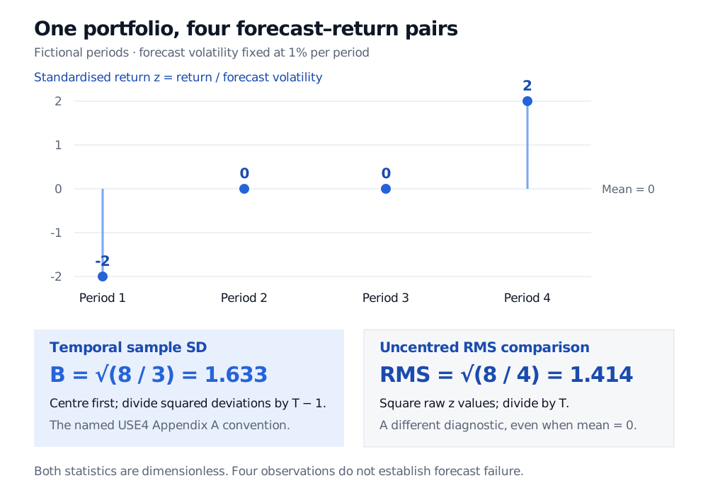
One fictional portfolio has standardised returns −2, 0, 0 and 2 over four periods. Their mean is zero. The temporal sample standard deviation is square root of 8 over 3, or 1.633; the uncentred RMS is square root of 8 over 4, or 1.414.
Original fictional example: the named temporal statistic and an RMS diagnostic use the same four observations but different denominators.
A high number is evidence to investigate
Four observations do not establish model failure. Under the specific null that the zt are independent and identically distributed normal observations with constant mean and population standard deviation one,
(T−1)B2∼χT−12.
This is the usual chi-squared variance-test construction described by NIST. For T=4, its central 95% reference range for B is approximately [0.2682,1.7653]. Our 1.6330 lies inside it. That range describes repeated samples under those assumptions; it is not a probability that this model is correct.
Serial dependence, overlapping return horizons, heavy tails and portfolios selected after examining their results change the inference. Normal-theory large-sample bands also need justification; enough observations alone do not make normal-theory coverage valid. A population dispersion target requires finite second moments. The usual iid variance-estimator asymptotics also assume finite fourth moments, as illustrated in Bates’s sample-variance example. Examining many portfolios or windows adds selection and multiple-testing concerns.
A long-window statistic can conceal opposite errors in successive regimes. Appendix A2 therefore examines rolling windows and mean rolling absolute deviation from one; its simulations show sensitivity to kurtosis. Overlapping windows are dependent.
The cross-sectional relative has a different job
USE4 also defines instantaneous cross-sectional bias measures for volatility regime adjustment, using squared standardised factor or specific returns across names at one date (§§4.3 and 5.3). Those measures and Appendix A's temporal sample standard deviation share a calibration idea, but their observations, weights and sampling behaviour differ. A large cross-section of correlated stocks is not automatically a large independent sample.
These are definitions from an August 2011 methodology document, not a description or guarantee of current vendor products.
For the forecast being checked, Risk Models: APT and Factor Structure derives the factor and specific components of portfolio variance. The full lesson requires membership; a public preview is available.